# Use built-in mtcars dataset for simplicity
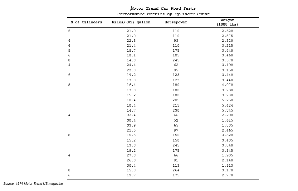
spec <- create_table(mtcars, cols = c(cyl, mpg, hp, wt)) |>
  add_title("Motor Trend Car Road Tests", styleRef = "i") |>
  add_title("Performance Metrics by Cylinder Count", styleRef = "i") |>
  add_footnote("Source: 1974 Motor Trend US magazine")

# Define columns with labels and styling
spec <- spec |>
  define_cols(c(mpg, hp, wt),
              label = c("Miles/(US) gallon", "Horsepower", "Weight<br>(1000 lbs)"),
              valueStyleRef = "ac"  # align center
              ) |>
  define_cols(cyl,
                        label = "N of Cylinders",
              dedupe = T) |>
    set_document(contentWidth = "60%")

# Create report and render to DOCX
report <- create_report(spec)
write_doc(report, name = "demo_table", outDir = "output")Getting Started with ksTFL: Creating Your First Clinical Table
R
ksTFL
Clinical Programming
A short intro to ksTFL R-Package to generate Clinical TFLs
Introduction
Creating clinical trial tables, figures, and listings is one of the most time-consuming tasks in clinical statistical programming. The ksTFL R Package was designed to make this process faster, more reliable, and more enjoyable.
In this post, we’ll walk through the basics of ksTFL and create your first clinical table.
Why ksTFL?
Clinical trial deliverables require:
- ✅ Professional formatting and alignment with regulatory standards
- ✅ Reproducible, auditable code
- ✅ Traceability of the data throughout the analysis pipeline
- ✅ Submission-ready output without manual refinement
Without a specialized tool, generating submission-ready tables and figures from R can require significant time—sometimes more than the time spent on statistical calculations and modeling itself.
Installation
Install ksTFL from r-universe:
Your First Table
Let’s create a simple demographic summary table using sample data:
What’s Happening?
create_table(data, cols = ...)- Initialize the table with selected columnsadd_title(),add_footnote()- Add documentation and annotationsdefine_cols()- Configure column properties (labels, styling, visibility, deduplication, etc.)create_report()- Assemble the table specificationwrite_doc()- Render to a professional DOCX document
With just a few lines of code, ksTFL generates a well-formatted MS Word DOCX document:
Key Features
Declarative Styling
Apply styles without modifying source data:
# Add conditional styling - highlight high horsepower
spec <- spec |>
  compute_cols(hp >=180,
               c_style(hp, styleRef = "fc_red"))  # font color red
The ksTFL package includes many pre-defined atomic styles, but custom styles can also be created using the add_style() function.
Spanning Headers
Create multi-column group headers:
spec <- spec |>
  add_span_header(cols = c(mpg, hp, wt),
                  label = "Performance Metrics")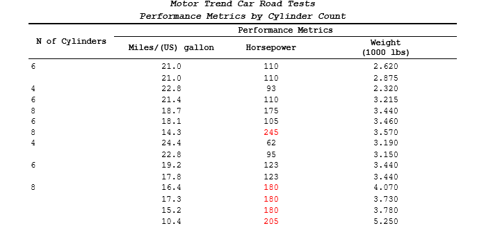
Flexible Column Selection
Use tidyselect helpers for column selection:
spec |>
  define_cols(starts_with("m"),
              valueStyleRef = "ar")  # right align
Built-in Style Atoms
Combine predefined styles for quick formatting:
# Combine multiple style attributes
spec <- add_title(spec, "Summary",
                  styleRef = f_combine("i", "b", "fc_navy"))
Complete Example: Demographics Table
Let’s build a submission-ready demographics table.
Since this article focuses on ksTFL’s rendering capabilities, the statistical calculations and data preparation are handled upstream. ksTFL does not calculate statistics by itself; rather, it transforms pre-calculated summary tables into publication-ready documents. In production code, statisticians prepare the summary data in a planar format, and ksTFL handles the table layout and formatting.
Below, we use a simple function that generates a data frame with calculated statistics for Age, Sex, and Race:
# Simple function that generates the summary table
# that a statistical programmer typically creates from ADSL data
generate_demography_summary <- function(seed = 1007L) {
    set.seed(seed)

    rnd_stat <- function(N) {
        c(
            sprintf("%.1f (%.1f)", rnorm(1L, 48, 2), rnorm(1L, 11, 1)),
            sprintf("%.1f", rnorm(1L, 49, 2)),
            sprintf("%d, %d", sample(20:30, 1L), sample(65:75, 1L)),
            sprintf("%d (%.1f%%)", 22L, 100 * 22L / N),
            sprintf("%d (%.1f%%)", 20L, 100 * 20L / N),
            sprintf("%d (%.1f%%)", 28L, 100 * 28L / N),
            sprintf("%d (%.1f%%)", 9L, 100 * 9L / N),
            sprintf("%d (%.1f%%)", 5L, 100 * 5L / N)
        )
    }

    data.frame(
        PARAM = c(rep("Age (years)",3), rep("Sex",2), rep("Race",3)),
        STATISTIC = c("Mean (SD)", "Median", "Min, Max",
                                    "Female", "Male",
                                    "White", "Asian", "Other"),
        PLACEBO = rnd_stat(placebo_n),
        DRUGA = rnd_stat(drug_a_n),
        TOTAL = rnd_stat(total_n),
        stringsAsFactors = FALSE
    )
}
With the inputs provided above, the generated data frame looks like this:
placebo_n <- 42L
drug_a_n <- 44L
total_n <- placebo_n + drug_a_n

table_data <- generate_demography_summary(seed = 1007L)

table_data
PARAM STATISTIC PLACEBO DRUGA TOTAL
1 Age (years) Mean (SD) 49.0 (11.3) 48.6 (9.8) 51.6 (12.1)
2 Age (years) Median 51.6 47.9 50.2
3 Age (years) Min, Max 26, 68 20, 75 26, 69
4 Sex Female 22 (52.4%) 22 (50.0%) 22 (25.6%)
5 Sex Male 20 (47.6%) 20 (45.5%) 20 (23.3%)
6 Race White 28 (66.7%) 28 (63.6%) 28 (32.6%)
7 Race Asian 9 (21.4%) 9 (20.5%) 9 (10.5%)
8 Race Other 5 (11.9%) 5 (11.4%) 5 (5.8%)Now let’s use ksTFL to transform this planar data frame into a submission-ready document:
# Initialize ksTFL table specification
table_spec <- create_table(table_data) |>
    # PARAM is set to invisible because we use it as a category header.
    # This keeps the table compact and maintains a professional appearance.
    define_cols(PARAM, label = "Parameter", isVisible = FALSE) |>
    # STATISTIC remains visible on every row because it distinguishes
    # different statistics within each parameter block.
    define_cols(STATISTIC,
                    label = "Parameter<br>Statistic",
                    valueStyleRef = "indent_1", labelStyleRef = 'al') |>
    # Treatment columns follow the same display rules, so we define them together.
    # Although ksTFL calculates column widths automatically,
    # we manually set them here to ensure consistent treatment column widths
    # across the output for visual clarity and professional presentation.
    define_cols(c(PLACEBO, DRUGA, TOTAL),
                            label = c(paste0("Placebo<br>(N=", placebo_n,')'),
                                                paste0("Drug A<br>(N=", drug_a_n,')'),
                                                paste0("Total<br>(N=", total_n,')')),
                            valueStyleRef = "ac",
                            colWidth = c("18%", "18%", "18%")
    ) |>
    compute_cols(
    # The input data lacks units for categorical statistics;
    # we add them dynamically here.
        PARAM %in% c('Sex', 'Race'),
        c_glue(PARAM, 'after', text=', n (%)')
    ) |>
    # Use PARAM values as heading rows for better structure
    compute_cols(
        firstOf(PARAM),
        c_addrow('above', value_from = PARAM, styleRef = f_combine('al', 'b'))
    ) |>
    # Define titles, subtitles, and document headers/footers
    add_title("Table 14.1 Demographic Summary") |>
    add_subtitle("(Safety Population)", styleRef = 'ac') |>
    add_footnote("Note: Values are presented as summary statistics prepared before the ksTFL stage.") |>
    add_header("Example Study KSTFL-107", "DEMOGRAPHY", "Page {PAGE} of {NUMPAGES}") |>
    add_footer("Basic summary table example", "", format(Sys.Date(), "%Y-%m-%d")) |>
    # Demographic tables benefit from a moderate content width:
    # narrow enough to keep treatment columns readable, but wide enough
    # to avoid sparse layouts with few rows.
    set_document(
        contentWidth = "50%",
        # ksTFL provides flexible control over footnote placement:
        # "doc_footer" (in the Word footer below footer rows),
        # "repeated" (under the table on every page), or
        # "last_page" (under the table on the last page only)
        footnotePlace = "doc_footer"
    )

# Create report and render to DOCX
report <- create_report(table_spec)

write_doc(report, name = "table_14_1", outDir = "output")
With just a few lines of declarative code, the planar data frame transforms into a production-ready document:
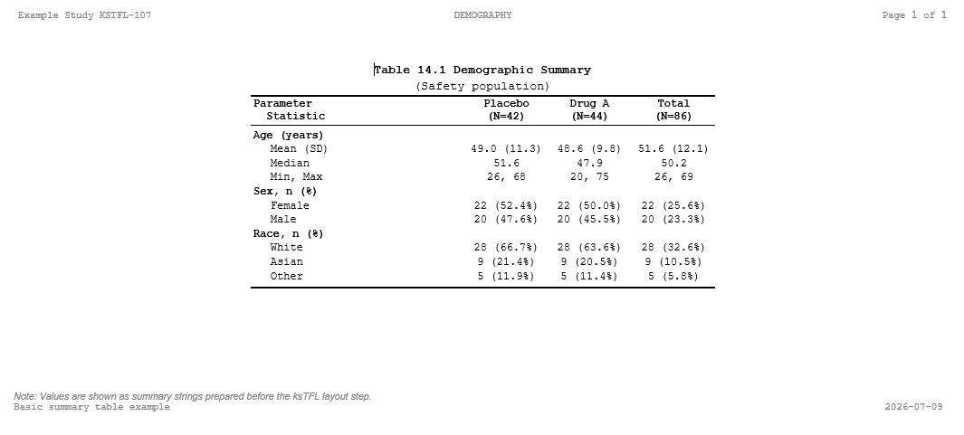
The key advantage of this approach is that the input data remains in a simple, planar format that is easy to validate and audit, without any embedded reporting artifacts or formatting logic.
Next Steps
Now that you understand the basics of ksTFL, you can:
- Explore the ksTFL Documentation for advanced features
- Check out the GitHub Repository for more real examples and scripts
- A LinkedIn Post here gives some additional context and background on the ksTFL package.
Aleschenkov I, Larchenko V (2026). ksTFL: Framework for Clinical Tables, Figures, and Listings. R package version 0.11.9, https://crow16384.github.io/ksTFL/ https://crow16384.r-universe.dev/ksTFL.
This post was originally published on the KeyStat Solutions Technical Blog. Visit R-Bloggers to discover more R content.