Tipping-Point Analysis under Multiple Imputation

Delta-adjust originally missing outcomes, Rubin-pool the treatment contrast, and assess robustness to specified MNAR departures

Clinical Trials

Data analysis

Missing Data

Data Imputation

Tipping Point

Author

Vladimir Larchenko

Published

September 4, 2026

Decorator architecture

Introduction

A tipping-point sensitivity analysis asks how far the assumptions about unobserved outcomes would have to depart from those used under MAR¹ before a pre-specified treatment conclusion changes. One practical implementation is controlled multiple imputation with a delta adjustment applied to originally missing outcomes, followed by re-analysis and Rubin pooling for each value of the sensitivity parameter (Ratitch, O’Kelly, and Tosiello, 2013; Cro, Morris, Kenward, and Carpenter, 2020).

In a clinical-trial setting, the interpretation of a tipping point depends on exactly how the sensitivity parameter is defined and on which path through the MNAR² sensitivity space is explored. A tipping point therefore does not by itself establish that MAR is plausible or implausible; it describes the departure from the MAR-based analysis required to cross a specified inferential boundary.

%%{init: {"theme": "base", "themeVariables": {"darkMode": false, "background": "#ffffff", "primaryColor": "#d6eaf8", "primaryTextColor": "#1a252f", "primaryBorderColor": "#1f6f8b", "lineColor": "#2c3e50", "mainBkg": "#d6eaf8", "titleColor": "#1a252f"}, "flowchart": {"padding": 10, "nodeSpacing": 14, "rankSpacing": 22, "curve": "linear"}}}%%
flowchart TD
  raw["Incomplete data"]
  mi["MAR MI once"]
  stack["MI datasets 1..M"]
  adj["Apply sensitivity-model delta<br/>to originally missing values"]
  fit["Fit primary analysis model;<br/>extract treatment contrast"]
  pool["Rubin-pool treatment contrast"]
  pval["Apply pre-specified<br/>inferential criterion"]
  raw --> mi --> stack --> adj --> fit --> pool --> pval
  classDef once fill:#d6eaf8,stroke:#1f6f8b,color:#1a252f,stroke-width:1.5px
  classDef each fill:#d5f5e3,stroke:#1e8449,color:#1a252f,stroke-width:1.5px
  class raw,mi,stack once
  class adj,fit,pool,pval each

There is an important terminology point first: the ordinary ANOVA³ F-test itself is not one-sided. For two treatment groups, the ANOVA test is equivalent to a two-sided \(t\)-test. A directional, one-sided hypothesis should therefore be expressed as a planned treatment contrast, e.g.

\[H_0 : \mu_D - \mu_P \leq 0 \quad \text{vs} \quad H_1 : \mu_D - \mu_P > 0.\]

That distinction becomes important for a tipping-point analysis.

Example setting

Suppose:

TRT = "DRUG" or "PLACEBO"
Y = primary endpoint (higher is better)
missing endpoint values are imputed under MAR
the primary analysis compares DRUG against PLACEBO
the test is one-sided in favor of DRUG.

Suppose the MAR estimate is

\[\Delta_{MAR} = \mu_D - \mu_P\]

The tipping-point analysis asks:

How unfavorable would the missing endpoint outcomes have to be, relative to MAR, along a specified sensitivity path, before the pre-specified one-sided statistical criterion is no longer met?

Delta adjustment

Delta-adjustment after MAR imputation is a controlled multiple-imputation sensitivity device: an offset is applied to imputed values to encode a clinically directed MNAR departure, then the primary analysis is repeated (Ratitch et al., 2013; Cro et al., 2020). For a higher-is-better endpoint, the unfavorable adjustment is

\[ Y_i^* = \begin{cases} Y_i^{MAR} - \delta, & i \in D, Y_i \text{ missing} \\ Y_i^{MAR} + \delta, & i \in P, Y_i \text{ missing} \\ Y_i, & \text{observed.} \end{cases} \]

So DRUG is made worse and PLACEBO is made better.

The word delta is then ambiguous. Two different quantities are often called \(\delta\), and they do not coincide.

What \(\delta\) can mean

The symbol \(\delta\) is potentially ambiguous because it can describe either a modification applied to individual missing observations or a desired change in the final treatment contrast. These are different quantities and should not be used interchangeably.

Definition A — arm-wise shift. \(\delta\) is the constant added to (or subtracted from) each originally missing observation. In the higher-is-better rule above, every missing DRUG value is lowered by \(\delta\) and every missing PLACEBO value is raised by \(\delta\). This is the definition used in the R code later.

Definition B — target change in the treatment contrast. Here \(\delta\) denotes the intended adverse change in the treatment contrast relative to the MAR analysis. This is a property of the analysis result, not necessarily the numerical offset applied to each missing observation. Saying “the tipping point is a \(100\,\mathrm{mL}\) adverse departure from MAR” often means Definition B: the pooled contrast itself has moved by about \(-100\,\mathrm{mL}\).

They are not interchangeable. The mapping between an arm-wise observation-level shift and a desired change in an adjusted treatment contrast generally depends on the analysis model and data structure. Therefore, a simple division by the missingness fraction is valid only under appropriately simple marginal-mean settings and should not be assumed for an ANCOVA or other adjusted model.

Why an arm-wise \(\delta\) is not a \(\delta\) change in \(\Delta\)

Consider first the simple case where the treatment effect is the unadjusted difference in overall arm means. Write \(\pi_D\) and \(\pi_P\) for the fractions of endpoint observations missing in the two arms. Observed values are never shifted, so an arm-wise shift of \(-\delta\) in missing DRUG observations and \(+\delta\) in missing PLACEBO observations changes the overall arm means by approximately

\[ \bar Y_D^\star - \bar Y_D^{\mathrm{MAR}} \approx -\pi_D\,\delta, \qquad \bar Y_P^\star - \bar Y_P^{\mathrm{MAR}} \approx +\pi_P\,\delta. \]

Therefore, for this simple marginal-mean analysis,

\[ \Delta^\star - \Delta_{\mathrm{MAR}} \approx -\delta(\pi_D+\pi_P). \]

This relationship is useful for explaining the scale of an arm-wise delta, but it should not be interpreted as a general formula for the change in an adjusted treatment effect.

In an ANCOVA or other model-based primary analysis, the treatment coefficient is a partial regression contrast. Its response to changing imputed outcomes depends on the covariates, design matrix, missingness pattern, and the fitted model. There is therefore generally no universal conversion such as

\[ \text{change in treatment coefficient} = -\delta(\pi_D+\pi_P). \]

For a model-based primary analysis, the effect of the sensitivity parameter on the treatment contrast should be determined by refitting the specified analysis model in every imputed dataset and then applying the appropriate MI combining rules.

Two special cases make the wording concrete for the unadjusted mean difference.

If all endpoint values were missing (\(\pi_D=\pi_P=1\)), then \(\Delta^\star-\Delta_{\mathrm{MAR}}\approx-2\delta\). One arm-wise unit produces a two-unit hit to the contrast: DRUG is lowered by \(\delta\) and PLACEBO is raised by \(\delta\).

If missingness is modest, the hit is smaller. With \(\pi_D=\pi_P=0.20\), an arm-wise \(\delta=100\,\mathrm{mL}\) moves the unadjusted contrast by only about \(-40\,\mathrm{mL}\). Calling that “a \(100\) mL tipping point” would overstate how far the treatment effect has been pushed.

If only the imputed means are discussed, not the overall arm means, the factor of two remains even when \(\pi<1\): the mean of the missing DRUG values is \(-\delta\) and the mean of the missing PLACEBO values is \(+\delta\), so their difference changes by \(-2\delta\). That is a statement about the MNAR departure among dropouts, not about \(\Delta\) in the ITT⁴ population.

What should be stated clearly

Any description of the sensitivity analysis should name both the operation and the meaning of the displayed \(\delta\).

Who is shifted. Only originally missing endpoint values, never observed values.
Direction. For a higher-is-better endpoint, DRUG missing values are worsened and PLACEBO missing values are improved (or only one arm is shifted; that must be said).
Scale of \(\delta\). Either
- “arm-wise: \(\delta\) mL is subtracted from each missing DRUG value and added to each missing PLACEBO value” (Definition A), or
- “contrast-wise: \(\delta\) is the target adverse change in \(\mu_D-\mu_P\)” (Definition B).
If Definition B is used, how it is implemented. For example, shift only missing DRUG values by \(\delta/\pi_D\), or split the contrast shift as \(\delta_D\) and \(\delta_P\) with \(\delta_D\pi_D+\delta_P\pi_P=\delta\). Without that map, the grid cannot be reproduced.

In a simple unadjusted mean-difference setting, the distinction can be illustrated numerically as follows. Suppose \(\Delta_{\mathrm{MAR}}=160\) mL, \(\pi_D=\pi_P=0.20\), and the one-sided test tips when the pooled contrast falls to \(80\) mL. That is a \(80\) mL adverse move in the treatment effect (Definition B). The corresponding arm-wise \(\delta\) (Definition A) is

\[ \delta_{\mathrm{arm}} \approx \frac{80}{\pi_D+\pi_P} = \frac{80}{0.40} = 200\,\mathrm{mL}. \]

Reporting “\(\delta_{\mathrm{TP}}=200\)” without saying arm-wise looks more extreme than reporting “the contrast was worsened by \(80\) mL”. Both numbers describe the same analysis. They answer different questions.

This article uses Definition A. Tables and plots are labelled as the arm-wise shift of originally missing FVC⁵. The two-dimensional grid later lets \(\delta_{\mathrm{DRUG}}\) and \(\delta_{\mathrm{PLACEBO}}\) differ, which is the honest way to avoid hiding the factor of two inside a single symbol.

Why every imputed dataset must be adjusted separately

Suppose you have \(M=50\) MI datasets:

\[D_1,D_2,\ldots,D_{50}.\]

You do not calculate one average imputed value and perform the tipping-point analysis on that.

Instead, for each delta:

\[\delta_1,\delta_2,\ldots,\delta_K\]

you create

\[D^{*}_{m,k}\]

for every combination of:

imputation \(m=1,\ldots,M\)
delta \(k=1,\ldots,K\).

So with 50 imputations and 11 delta values, you have

\[50\times11=550\]

analyses.

For each fixed delta, the 50 treatment-effect estimates are combined using MI rules.

This preserves the between-imputation component of uncertainty required by the multiple-imputation combining rules. Multiple imputation is specifically intended to retain between-imputation variability rather than treating one completed dataset as if it were the truth.

The statistical procedure

For a given \(\delta\):

Step 1 — Analyze each imputed dataset

For imputation \(m\), fit for example

\[Y^*=\beta_0 + \beta_1 TRT + \beta_2 Y_{\mathrm{baseline}} + \varepsilon\]

That is usually more representative of a clinical-trial primary analysis than a simple one-way ANOVA.

Step 2 — Rubin pooling

For \(M\) imputations, Rubin’s rules (Rubin, 1987) give

\[\bar\beta(\delta) = \frac{1}{M}\sum^M_{m=1}\hat\beta_m(\delta)\]

and

\[\bar U(\delta) = \frac{1}{M}\sum_m U_m(\delta).\]

The between-imputation variance is

\[B(\delta) = \frac{1}{M-1}\sum_m \Big[\hat \beta_m(\delta)-\bar \beta(\delta)\Big]^2\]

Then the total variance is

\[T(\delta) = \bar U(\delta) + \Big(1+\frac{1}{M}\Big)B(\delta)\]

Thus

\[SE(\delta) = \sqrt{T(\delta)}\]

The degrees of freedom are obtained using the MI combining rules. Modern implementations of mice::pool() use the Barnard–Rubin (1999) MI-adjusted degrees of freedom rather than simply using the complete-data residual df.

One-sided p-value

Suppose the efficacy hypothesis is

\[H_1: \beta_1 > 0.\]

Then

\[p_{one-sided} = 1 - F_{t,\nu}(t(\delta))\]

where \(F_{t,\nu}\) is the \(t\) CDF with MI-adjusted degrees of freedom.

So if your significance level is

\[\alpha=0.025,\]

you declare that the specified statistical criterion is met at a particular delta if

\[p_{\text{one-sided}}(\delta)<0.025.\]

Equivalently,

\[t(\delta) > t_{0.975,\nu}.\]

What is the tipping point?

A tipping point must always be defined relative to:

the sensitivity parameterization;
the direction of the adverse departure;
the analysis model;
the inferential criterion; and
the path or region of sensitivity values being explored.

In this article, the one-dimensional tipping point is defined as the first value along the symmetric arm-wise path

\[\delta_D=\delta_P=\delta,\]

where missing DRUG outcomes are decreased by \(\delta\) and missing PLACEBO outcomes are increased by \(\delta\), for which the pre-specified one-sided test no longer satisfies

\[p_{\text{one-sided}} < 0.025.\]

Thus the reported tipping point is not a universal property of the data. It is a property of the data under this particular sensitivity model and inferential rule.

Imagine the following results:

\(\delta\)	pooled estimate	one-sided p
0	5.2	0.003
1	4.0	0.008
2	2.8	0.019
3	1.6	0.047
4	0.4	0.31

Then the tipping point lies between

\[\delta=2\]

and

\[\delta=3\]

The interpretation is roughly:

Under the MAR analysis, the treatment comparison meets the specified one-sided statistical criterion. That criterion ceases to be met when the missing DRUG outcomes are sufficiently worsened and the missing PLACEBO outcomes sufficiently improved by approximately this delta along the symmetric arm-wise path.

Usually one reports the smallest delta at which the one-sided test fails, together with the corresponding treatment estimate, SE, CI and p-value. The grid interval should remain part of the reported result; a numerical crossing (e.g. from uniroot()) is a refinement of that interval, not an estimated biological parameter.

Statistical versus clinical tipping points

The tipping point used in this article is defined by statistical significance:

\[p_{\text{one-sided}} \ge 0.025.\]

A different and often clinically useful question is when the treatment effect ceases to exceed a pre-specified clinically relevant threshold \(M\):

\[H_0:\beta_1\le M \quad\text{vs}\quad H_1:\beta_1>M.\]

The corresponding sensitivity boundary would answer a different question: how much departure from MAR is required before the treatment effect no longer provides evidence of exceeding the clinically relevant threshold?

These two tipping points need not be the same. A result can remain clinically large while losing statistical significance, or remain statistically significant while falling below a clinically meaningful target.

What the tipping point does NOT tell you

A tipping-point analysis does not estimate the probability that the data are MNAR, nor does it establish the true value of the sensitivity parameter.

It does not show that MAR is true when \(\delta=0\), nor that an MNAR departure of \(\delta_{\mathrm{TP}}\) is clinically plausible.

It does not mean that the treatment effect changes by exactly \(\delta_{\mathrm{TP}}\).

It does not establish that efficacy disappears at the tipping point. It establishes only that the specified statistical decision rule changes at that point.

Its value comes from comparing the required departure from MAR with scientifically credible and clinically plausible departures.

R implementation

Here is a fairly direct implementation using mice.

Suppose imp is your mids object.

First preserve the original missingness indicator:

dat <- imp$data

dat$miss_y <- is.na(dat$Y)

This is crucial.

You want to adjust only values that were originally missing and subsequently imputed.

You must not do this:

Y = Y - delta

because that changes observed values too.

Extract all imputed datasets

library(mice)
library(dplyr)

imp_data <- complete(imp, action = "all")

mice supports working with the collection of completed imputations, and its tooling distinguishes observed from imputed values.

Delta adjustment

For higher-is-better:

make_tipping_data <- function(data, delta) {

  data %>%
    mutate(
      Y_tp = case_when(
        miss_y & TRT == "DRUG"    ~ Y - delta,
        miss_y & TRT == "PLACEBO" ~ Y + delta,
        TRUE ~ Y
      )
    )
}

Then:

delta_grid <- seq(0, 5, by = 0.5)

Analyze each imputed dataset

For a simple two-arm comparison:

fit_one <- function(data) {

  lm(
    Y_tp ~ TRT,
    data = data
  )
}

For a treatment contrast, make PLACEBO the reference:

data$TRT <- relevel(factor(data$TRT), ref = "PLACEBO")

Then the coefficient of TRTDRUG is

\[\hat\mu_D - \hat\mu_P.\]

Pool the 50 analyses for one delta

You can fit each completed dataset separately and turn the results into a mira object:

library(mice)

fit_and_pool <- function(datasets, delta) {

  fits <- lapply(datasets, function(dat) {

    dat <- make_tipping_data(dat, delta)

    dat$TRT <- relevel(
      factor(dat$TRT),
      ref = "PLACEBO"
    )

    lm(Y_tp ~ TRT, data = dat)
  })

  pooled <- pool(as.mira(fits))

  pooled
}

Then:

pooled <- fit_and_pool(imp_data, delta = 2)
summary(pooled)

Obtain the one-sided p-value

summary(pool(...)) ordinarily gives the usual two-sided p-value.

For the treatment coefficient:

s <- summary(pooled)

trt_row <- s[s$term == "TRTDRUG", ]

t_stat <- trt_row$estimate / trt_row$std.error
df     <- trt_row$df

p_one <- 1 - pt(t_stat, df)

c(
  estimate = trt_row$estimate,
  SE       = trt_row$std.error,
  df       = df,
  t        = t_stat,
  p_one    = p_one
)

For

\[H_1: DRUG > PLACEBO,\]

this is the appropriate tail.

Run the complete tipping-point grid

library(purrr)
library(tibble)

tip_results <- map_dfr(delta_grid, function(delta) {

  fits <- lapply(imp_data, function(dat) {

    dat <- make_tipping_data(dat, delta)

    dat$TRT <- relevel(
      factor(dat$TRT),
      ref = "PLACEBO"
    )

    lm(Y_tp ~ TRT, data = dat)
  })

  pooled <- pool(as.mira(fits))
  s <- summary(pooled)

  z <- s[s$term == "TRTDRUG", ]

  t_stat <- z$estimate / z$std.error

  tibble(
    delta    = delta,
    estimate = z$estimate,
    SE       = z$std.error,
    df       = z$df,
    t        = t_stat,
    p_one    = 1 - pt(t_stat, z$df)
  )
})

You then get something like:

# A tibble:
  delta estimate    SE    df     t   p_one
   0.0    5.21    1.74  86.4  2.99  0.002
   0.5    4.60    1.76  85.8  2.61  0.005
   1.0    4.01    1.78  84.7  2.25  0.013
   1.5    3.40    1.80  82.9  1.89  0.031
   2.0    2.82    1.82  81.5  1.55  0.063

Therefore the significance boundary on the arm-wise delta scale lies between 1.5 and 2.0.

Find the tipping point numerically

Instead of restricting yourself to a coarse grid, you can locate the crossing of the implemented one-sided \(p\)-value function more precisely — but only after the grid has identified a bracketing interval.

A root finder should only be used when the chosen interval brackets a crossing and the sensitivity function behaves appropriately over that interval. In a general application, the one-sided \(p\)-value need not be globally monotone in the sensitivity parameter. The grid should therefore be used first to identify and verify the relevant crossing rather than assuming that uniroot() can safely be applied to an arbitrary interval.

For example:

tip_results %>%
  filter(p_one >= 0.025) %>%
  slice_min(delta)

This gives the first delta on your grid where significance is lost.

For a report, show both:

Delta grid: 0, 0.25, 0.50, ..., 5.00

and identify the interval

\[\delta_{TP}\in[\delta_L,\delta_U]\]

One more subtle issue: ANOVA vs treatment contrast

If the actual analysis is:

lm(Y ~ TRT)

with two groups, then

\[F=t^2.\]

The F-test answers

\[H_0: \mu_D=\mu_P\]

without direction.

For a one-sided efficacy claim, extract the DRUG-versus-PLACEBO coefficient and calculate the one-sided test.

For example:

fit <- lm(Y_tp ~ TRT, data = dat)

beta <- coef(fit)["TRTDRUG"]

and then pool beta.

If your actual primary analysis has baseline adjustment, LS-means, strata, site effects, repeated measurements, etc., the same tipping-point architecture remains valid, but the model inside each imputation should be exactly the primary analysis model.

The complete conceptual picture

%%{init: {"theme": "base", "themeVariables": {"darkMode": false, "background": "#ffffff", "primaryColor": "#d6eaf8", "primaryTextColor": "#1a252f", "primaryBorderColor": "#1f6f8b", "lineColor": "#2c3e50", "mainBkg": "#d6eaf8", "clusterBkg": "#f7f9fb", "clusterBorder": "#5d6d7e", "titleColor": "#1a252f"}, "flowchart": {"padding": 10, "nodeSpacing": 14, "rankSpacing": 26, "curve": "linear"}}}%%
flowchart TD
  raw["Original incomplete data"]
  mi["MAR multiple imputation once"]
  stack["Completed MI datasets 1..M"]
  delta0["Start at delta = 0"]
  adj["Apply specified sensitivity-model delta<br/>to originally missing values"]
  fit["Fit the primary analysis model;<br/>extract the pre-specified treatment contrast"]
  pool["Rubin-pool the M treatment contrasts"]
  pval["Apply pre-specified inferential criterion"]
  ask{"Criterion not met?"}
  tip["SENSITIVITY BOUNDARY"]
  more["Increase delta"]
  raw --> mi --> stack --> delta0 --> adj --> fit --> pool --> pval --> ask
  ask -->|yes| tip
  ask -->|no| more --> adj
  classDef step fill:#d6eaf8,stroke:#1f6f8b,color:#1a252f,stroke-width:1.5px
  classDef stopc fill:#fdebd0,stroke:#b9770e,color:#1a252f,stroke-width:1.5px
  classDef good fill:#d5f5e3,stroke:#1e8449,color:#1a252f,stroke-width:1.5px
  class raw,mi,stack,delta0,adj,fit,pool,pval,more step
  class ask stopc
  class tip good

The most important methodological principle is therefore:

\[\boxed{ \text{For each }\delta,\; \text{adjust all }M\text{ imputed datasets separately, analyze all }M, \text{ then pool.} }\]

That is the part that makes a multiple-imputation tipping-point analysis fundamentally different from simply modifying one completed dataset.

If the actual primary analysis is ANOVA with LSMeans/contrast (e.g. SAS PROC MIXED/GLIMMIX) rather than lm(Y ~ TRT), the same tipping-point procedure can be implemented with emmeans and Rubin pooling, which is closer to how many primary analyses are reported in practice.

Worked example: simulated FVC trial

The methods above are now applied to a simulated two-arm study whose primary efficacy variable \(Y\) is forced vital capacity (FVC), in millilitres. Higher FVC is better, so the one-sided claim remains

\[H_0:\mu_D-\mu_P\le 0\quad\text{vs}\quad H_1:\mu_D-\mu_P>0.\]

Gender (SEX) enters both the imputation model and the analysis model as a factor. The analysis inside every completed dataset is the ANCOVA

\[\mathrm{FVC}=\beta_0+\beta_1\mathrm{TRT}+\beta_2\mathrm{FVC}_{\mathrm{bl}}+\beta_3\mathrm{SEX}+\varepsilon.\]

With PLACEBO as the reference level, \(\beta_1\) is the gender- and baseline-adjusted DRUG-versus-PLACEBO contrast. Because the sensitivity analysis changes the outcome values and then refits the ANCOVA, the relationship between the arm-wise delta and the resulting treatment coefficient is determined empirically by the fitted model. The simple missingness-fraction formula given earlier should not be used to predict the ANCOVA coefficient.

The steps below follow that pipeline: simulate complete FVC, impose MAR missingness, impute with mice, delta-adjust each imputation, pool with Rubin’s rules, then read the tipping point from the one-sided \(p\)-value curve.

Setup

Packages used for wrangling, imputation, pooling, and graphics:

library(mice)


Attaching package: 'mice'

The following object is masked from 'package:stats':

    filter

The following objects are masked from 'package:base':

    cbind, rbind

library(dplyr, warn.conflicts = FALSE)
library(ggplot2)
library(purrr)
library(tibble)
library(tidyr)

set.seed(45672)
alpha_one <- 0.025

set.seed(45672) makes the simulated trial, the missingness indicators, and the PMM draws reproducible.

Step 1 — Simulate complete FVC data

A complete-data trial is generated first so that missingness can be imposed afterwards under a known MAR mechanism. Design choices:

\(N=200\), 1:1 randomisation to DRUG or PLACEBO.
About 40% female; males have a higher baseline FVC (about +800 mL), as in adult spirometry.
The data-generating mechanism specifies an expected treatment difference of approximately 160 mL in FVC change, with placebo declining more than DRUG. Because the trial is simulated with random error, the realized sample treatment difference will not be exactly 160 mL.
Residual SD is 250 mL, which is in a plausible range for FVC change in patients with some lung disease.

FVC_true is the complete endpoint value. It is kept only for diagnostics and is not used in imputation or in the tipping-point model.

n <- 200

dat_complete <- tibble(
  SUBJID = sprintf("S%03d", seq_len(n)),
  TRT    = factor(rep(c("PLACEBO", "DRUG"), each = n / 2),
                  levels = c("PLACEBO", "DRUG")),
  SEX    = factor(
    rbinom(n, 1, 0.40),
    levels = c(0, 1),
    labels = c("M", "F")
  )
) %>%
  mutate(
    FVC_bl = 2750 +
      if_else(SEX == "F", -800, 0) +
      rnorm(n(), sd = 400),
    decline = if_else(TRT == "DRUG", 50, 210) + rnorm(n(), sd = 250),
    FVC_true = FVC_bl - decline
  )

dat_complete %>%
  group_by(TRT, SEX) %>%
  summarise(
    n        = n(),
    FVC_bl   = mean(FVC_bl),
    FVC    = mean(FVC_true),
    change   = mean(FVC_true - FVC_bl),
    .groups  = "drop"
  )

# A tibble: 4 × 6
  TRT     SEX       n FVC_bl   FVC change
  <fct>   <fct> <int>  <dbl> <dbl>  <dbl>
1 PLACEBO M        63  2688. 2494. -195. 
2 PLACEBO F        37  1871. 1674. -197. 
3 DRUG    M        62  2870. 2823.  -47.1
4 DRUG    F        38  1969. 1876.  -92.7

The complete-data treatment contrast is the difference in mean endpoint FVC after accounting for the larger male lungs and the larger placebo decline. Gender is a factor, not a numeric 0/1 covariate in the analysis model, so the later lm() dummy-coding stays explicit.

Step 2 — Impose MAR missingness on endpoint FVC

Only endpoint FVC is allowed to be missing. The probability of a missing endpoint value depends on observed variables (TRT, FVC_bl, SEX) and not on FVC_true. This missingness mechanism is MAR by construction because the probability of missingness depends on variables that remain observed rather than on the unobserved endpoint itself. The specified mice imputation model is designed to be compatible with that MAR assumption.

More generally, mice is a framework for specifying multiple-imputation models; MAR is an assumption about the relationship between the missingness mechanism and the observed/unobserved data, not a property that is automatically guaranteed by using mice.

The logistic missingness model is tilted so that dropout is higher on PLACEBO, higher at lower baseline FVC, and slightly higher in females. The intercept is chosen so that the overall missingness rate is about 15–25%.

dat <- dat_complete %>%
  mutate(
    lp_miss = -1.70 +
      0.55 * (TRT == "PLACEBO") +
      0.22 * (SEX == "F") +
      0.0007 * (2400 - FVC_bl),
    p_miss  = plogis(lp_miss),
    miss_fvc = rbinom(n(), 1, p_miss) == 1,
    FVC = if_else(miss_fvc, NA_real_, FVC_true)
  )

dat %>%
  group_by(TRT, SEX) %>%
  summarise(
    n       = n(),
    n_miss  = sum(miss_fvc),
    pct_miss = 100 * mean(miss_fvc),
    .groups = "drop"
  )

# A tibble: 4 × 5
  TRT     SEX       n n_miss pct_miss
  <fct>   <fct> <int>  <int>    <dbl>
1 PLACEBO M        63      9     14.3
2 PLACEBO F        37     12     32.4
3 DRUG    M        62      9     14.5
4 DRUG    F        38      9     23.7

miss_fvc is stored before imputation. Later delta-adjustment uses this flag, not is.na(FVC) on a completed dataset, because after mice every FVC value is filled in.

p_miss_overall <- mean(dat$miss_fvc)
p_miss_overall

[1] 0.195

Step 3 — Describe the incomplete data

Two plots check that the simulation looks like a small FVC trial: missingness differs by arm and gender, and the observed endpoint distributions still show a DRUG advantage among completers.

miss_plot_dat <- dat %>%
  count(TRT, SEX, miss_fvc) %>%
  group_by(TRT, SEX) %>%
  mutate(pct = 100 * n / sum(n)) %>%
  ungroup() %>%
  filter(miss_fvc)

ggplot(miss_plot_dat, aes(x = TRT, y = pct, fill = SEX)) +
  geom_col(position = position_dodge(width = 0.8), width = 0.7) +
  labs(
    title = "MAR missingness for endpoint FVC",
    x = "Treatment",
    y = "Missing endpoint FVC (%)",
    fill = "Gender"
  ) +
  theme_bw()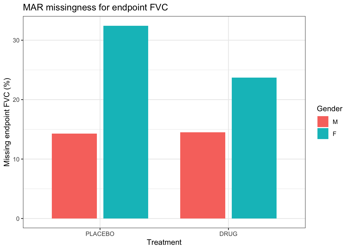

Figure 1: Percent of subjects with missing endpoint FVC, by treatment and gender.

ggplot(
  dat %>% filter(!miss_fvc),
  aes(x = TRT, y = FVC, fill = SEX)
) +
  geom_violin(alpha = 0.35, colour = NA) +
  geom_boxplot(width = 0.18, outlier.shape = NA, alpha = 0.85) +
  labs(
    title = "Observed endpoint FVC (completers)",
    x = "Treatment",
    y = "Endpoint FVC (mL)",
    fill = "Gender"
  ) +
  theme_bw()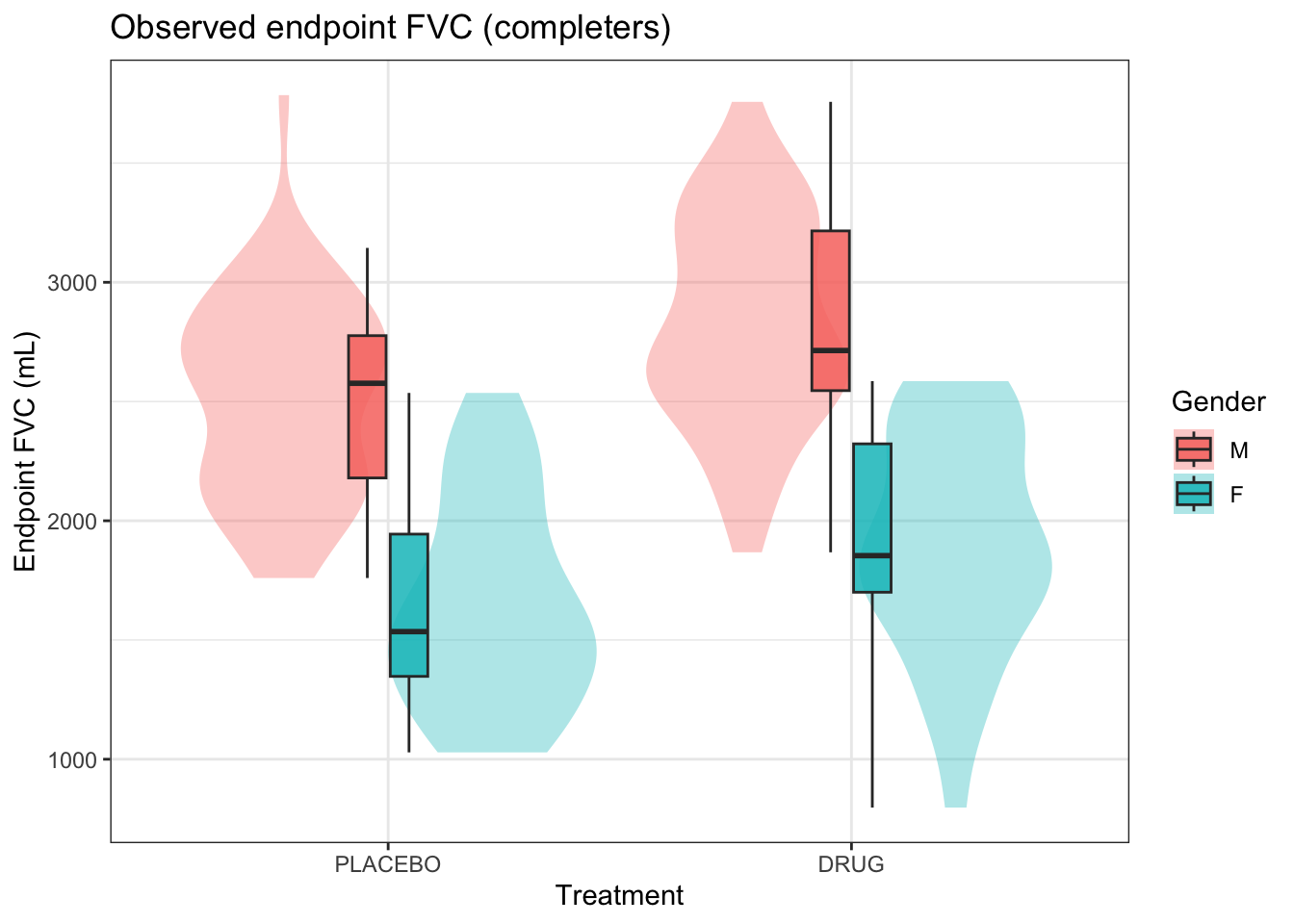

Figure 2: Observed endpoint FVC among completers, by treatment and gender.

Observed-case means are not the primary analysis. They are shown only to confirm that the generated FVC values and the MAR dropout pattern are in a sensible range.

Step 4 — MAR multiple imputation with `mice`

FVC is the only incomplete analysis variable. Predictors are TRT, FVC_bl, and SEX. Including gender in the imputation model matters because males and females have different FVC levels; omitting it would impute toward a pooled mean and distort both arms.

SUBJID and FVC_true are excluded as predictors. FVC_true would leak the complete outcome and would no longer be a realistic MAR analysis.

Predictive mean matching (pmm) is used so that the MAR-imputed endpoint values are selected from observed donor values and therefore remain on the observed outcome support (van Buuren, 2018). The subsequent delta adjustment is a separate sensitivity operation and can intentionally move those imputed values outside the observed support. \(M=50\) imputations retain between-imputation variance for Rubin’s rules.

dat_mi <- dat %>%
  select(TRT, SEX, FVC_bl, FVC)

pred <- make.predictorMatrix(dat_mi)
pred[, ] <- 0
pred["FVC", c("TRT", "SEX", "FVC_bl")] <- 1

meth <- make.method(dat_mi)
meth[] <- ""
meth["FVC"] <- "pmm"

imp <- mice(
  dat_mi,
  m               = 50,
  method          = meth,
  predictorMatrix = pred,
  printFlag       = FALSE,
  seed            = 3456
)

imp

Class: mids
Number of multiple imputations:  50 
Imputation methods:
   TRT    SEX FVC_bl    FVC 
    ""     ""     ""  "pmm" 
PredictorMatrix:
       TRT SEX FVC_bl FVC
TRT      0   0      0   0
SEX      0   0      0   0
FVC_bl   0   0      0   0
FVC      1   1      1   0

Completed datasets are extracted as a list. The original missingness flag is joined back onto every imputation so that later adjustments touch only originally missing the endpoint values.

imp_data <- complete(imp, action = "all") %>%
  map(~ mutate(.x, miss_fvc = dat$miss_fvc, SUBJID = dat$SUBJID))

Step 5 — Analysis and pooling helpers

The following functions implement the architecture from the methods section, now with FVC names and gender in the ANCOVA.

make_tipping_data() applies the higher-is-better MNAR shift: missing DRUG FVC is reduced by \(\delta\), missing PLACEBO FVC is increased by \(\delta\), observed values are left unchanged.
fit_ancova() fits \(\mathrm{FVC}^{\mathrm{TP}}\sim\mathrm{TRT}+\mathrm{FVC}_{\mathrm{bl}}+\mathrm{SEX}\) with PLACEBO as the reference.
pool_one_delta() analyses all \(M\) imputations at a given \(\delta\) (or at a pair of arm-specific deltas) and returns the Rubin-pooled treatment contrast and the one-sided \(p\)-value.

make_tipping_data <- function(data, delta, delta_drug = NULL, delta_pbo = NULL) {
  d_drug <- if (is.null(delta_drug)) delta else delta_drug
  d_pbo  <- if (is.null(delta_pbo)) delta else delta_pbo

  data %>%
    mutate(
      FVC_tp = case_when(
        miss_fvc & TRT == "DRUG"    ~ FVC - d_drug,
        miss_fvc & TRT == "PLACEBO" ~ FVC + d_pbo,
        TRUE ~ FVC
      )
    )
}

fit_ancova <- function(data) {
  data$TRT <- relevel(factor(data$TRT), ref = "PLACEBO")
  data$SEX <- factor(data$SEX, levels = c("M", "F"))
  lm(FVC_tp ~ TRT + FVC_bl + SEX, data = data)
}

pool_one_delta <- function(datasets, delta = 0, delta_drug = NULL, delta_pbo = NULL) {
  fits <- lapply(datasets, function(dat) {
    dat <- make_tipping_data(dat, delta, delta_drug, delta_pbo)
    fit_ancova(dat)
  })

  pooled <- pool(as.mira(fits))
  s <- summary(pooled)
  z <- s[s$term == "TRTDRUG", ]

  delta    = if (is.null(delta_drug) && is.null(delta_pbo)) delta else NA_real_
  delta_drug = if (is.null(delta_drug)) delta else delta_drug
  delta_pbo  = if (is.null(delta_pbo)) delta else delta_pbo
  
  tibble(
    delta = delta,
    delta_drug = delta_drug,
    delta_pbo = delta_pbo,
    estimate = z$estimate,
    SE       = z$std.error,
    df       = z$df,
    t        = z$estimate / z$std.error,
    p_one    = 1 - pt(z$estimate / z$std.error, z$df),
    ci_lo    = z$estimate - qt(0.975, z$df) * z$std.error,
    ci_hi    = z$estimate + qt(0.975, z$df) * z$std.error
  )
}

\(\delta=0\) is the ordinary MAR analysis: no MNAR shift, only mice imputation and the ANCOVA with gender.

mar_result <- pool_one_delta(imp_data, delta = 0)
mar_result

# A tibble: 1 × 10
  delta delta_drug delta_pbo estimate    SE    df     t     p_one ci_lo ci_hi
  <dbl>      <dbl>     <dbl>    <dbl> <dbl> <dbl> <dbl>     <dbl> <dbl> <dbl>
1     0          0         0     173.  40.1  139.  4.32 0.0000146  94.0  253.

If p_one at \(\delta=0\) is below 0.025, the MAR conclusion is that the specified one-sided statistical criterion is met for the DRUG-versus-PLACEBO contrast. The tipping-point question is how large an adverse shift of the imputed values is needed before that criterion is no longer met.

Step 6 — One-dimensional tipping-point grid

A grid of arm-wise deltas from 0 to 300 mL is applied along the symmetric path \(\delta_D=\delta_P=\delta\). This is a deliberately chosen sensitivity path through a two-dimensional MNAR space, not a uniquely defined representation of MNAR. For each \(\delta\), all 50 imputations are adjusted, the ANCOVA is fitted 50 times, and Rubin’s rules are applied before the one-sided test. That is 13 × 50 = 650 fitted models, not one adjusted dataset.

delta_grid <- seq(0, 300, by = 25)

tip_results <- map_dfr(delta_grid, function(d) {
  pool_one_delta(imp_data, delta = d)
})

tip_results

# A tibble: 13 × 10
   delta delta_drug delta_pbo estimate    SE    df     t     p_one  ci_lo ci_hi
   <dbl>      <dbl>     <dbl>    <dbl> <dbl> <dbl> <dbl>     <dbl>  <dbl> <dbl>
 1     0          0         0    173.   40.1  139.  4.32 0.0000146  94.0   253.
 2    25         25        25    164.   40.1  139.  4.09 0.0000367  84.6   243.
 3    50         50        50    154.   40.2  139.  3.85 0.0000906  75.1   234.
 4    75         75        75    145.   40.3  140.  3.60 0.000218   65.5   225.
 5   100        100       100    136.   40.4  140.  3.36 0.000509   55.7   216.
 6   125        125       125    126.   40.6  141.  3.11 0.00114    45.9   207.
 7   150        150       150    117.   40.9  142.  2.86 0.00246    36.0   198.
 8   175        175       175    107.   41.2  143.  2.61 0.00504    26.0   189.
 9   200        200       200     98.0  41.6  143.  2.36 0.00983    15.9   180.
10   225        225       225     88.6  42.0  145.  2.11 0.0182      5.71  172.
11   250        250       250     79.2  42.4  146.  1.87 0.0318     -4.57  163.
12   275        275       275     69.8  42.9  147.  1.63 0.0528    -14.9   155.
13   300        300       300     60.4  43.4  148.  1.39 0.0831    -25.4   146.

The first grid point at which the one-sided test fails (\(p \ge 0.025\)) brackets the significance boundary from above. A linear interpolation on the \(p\)-value (or on the \(t\) statistic) between the last significant and first non-significant grid points gives a finer numerical location of the crossing along the symmetric arm-wise path.

last_sig <- tip_results %>%
  filter(p_one < alpha_one) %>%
  slice_max(delta, n = 1)

first_ns <- tip_results %>%
  filter(p_one >= alpha_one) %>%
  slice_min(delta, n = 1)

if (nrow(last_sig) == 1 && nrow(first_ns) == 1) {
  delta_tp <- approx(
    x    = c(last_sig$p_one, first_ns$p_one),
    y    = c(last_sig$delta, first_ns$delta),
    xout = alpha_one
  )$y
} else if (nrow(first_ns) == 0) {
  delta_tp <- NA_real_
} else {
  delta_tp <- first_ns$delta
}

list(
  last_significant = last_sig,
  first_nonsignificant = first_ns,
  delta_tp_interpolated = delta_tp
)

$last_significant
# A tibble: 1 × 10
  delta delta_drug delta_pbo estimate    SE    df     t  p_one ci_lo ci_hi
  <dbl>      <dbl>     <dbl>    <dbl> <dbl> <dbl> <dbl>  <dbl> <dbl> <dbl>
1   225        225       225     88.6  42.0  145.  2.11 0.0182  5.71  172.

$first_nonsignificant
# A tibble: 1 × 10
  delta delta_drug delta_pbo estimate    SE    df     t  p_one ci_lo ci_hi
  <dbl>      <dbl>     <dbl>    <dbl> <dbl> <dbl> <dbl>  <dbl> <dbl> <dbl>
1   250        250       250     79.2  42.4  146.  1.87 0.0318 -4.57  163.

$delta_tp_interpolated
[1] 237.4919

A direct root finder on the pooled one-sided \(p\)-value is used when the grid straddles 0.025. The grid establishes that the significance boundary lies between consecutive grid points; uniroot() then locates the crossing of the implemented sensitivity-analysis function more precisely. This evaluates a few extra \(\delta\) values but does not replace the grid, which remains the reportable display. The numerical value should be interpreted as a numerical location of the decision boundary in the specified sensitivity model, not as an estimated clinical or biological parameter with a confidence interval.

p_one_at <- function(d) {
  pool_one_delta(imp_data, delta = d)$p_one
}

if (nrow(last_sig) == 1 && nrow(first_ns) == 1) {
  delta_tp_exact <- uniroot(
    function(d) p_one_at(d) - alpha_one,
    interval = c(last_sig$delta, first_ns$delta)
  )$root
} else {
  delta_tp_exact <- delta_tp
}

delta_tp_exact

[1] 238.922

Step 7 — Tipping-point graphics

The \(p\)-value curve shows when the one-sided test crosses \(\alpha=0.025\). The estimate curve shows the same information on the FVC (mL) scale, with Rubin-pooled 95% confidence intervals. The vertical line marks the numerically determined crossing of the one-sided significance threshold for the specified arm-wise sensitivity path.

p_plot <- ggplot(tip_results, aes(x = delta, y = p_one)) +
  geom_hline(yintercept = alpha_one, linetype = "dashed") +
  geom_line() +
  geom_point() +
  labs(
    title = "One-sided p-value versus symmetric arm-wise delta",
    subtitle = "DRUG missing: −δ; PLACEBO missing: +δ; dashed: α = 0.025; dotted: numerical crossing",
    x = "Arm-wise delta applied to originally missing endpoint FVC (mL)",
    y = "One-sided p-value (DRUG > PLACEBO)"
  ) +
  theme_bw()

if (is.finite(delta_tp_exact)) {
  p_plot <- p_plot + geom_vline(xintercept = delta_tp_exact, linetype = "dotted")
}
p_plot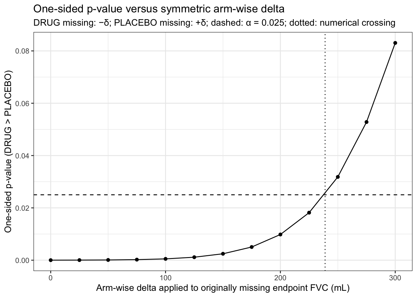

Figure 3: One-sided p-value versus the symmetric arm-wise delta applied to originally missing endpoint FVC.

est_plot <- ggplot(tip_results, aes(x = delta, y = estimate)) +
  geom_hline(yintercept = 0, linetype = "dashed") +
  geom_ribbon(aes(ymin = ci_lo, ymax = ci_hi), alpha = 0.18) +
  geom_line() +
  geom_point() +
  labs(
    title = "Rubin-pooled treatment contrast versus symmetric arm-wise delta",
    subtitle = "Ribbon: Rubin-pooled 95% CI; higher FVC is better",
    x = "Symmetric arm-wise delta applied to originally missing FVC (mL)",
    y = "Rubin-pooled adjusted DRUG − PLACEBO contrast (mL)"
  ) +
  theme_bw()

if (is.finite(delta_tp_exact)) {
  est_plot <- est_plot + geom_vline(xintercept = delta_tp_exact, linetype = "dotted")
}
est_plot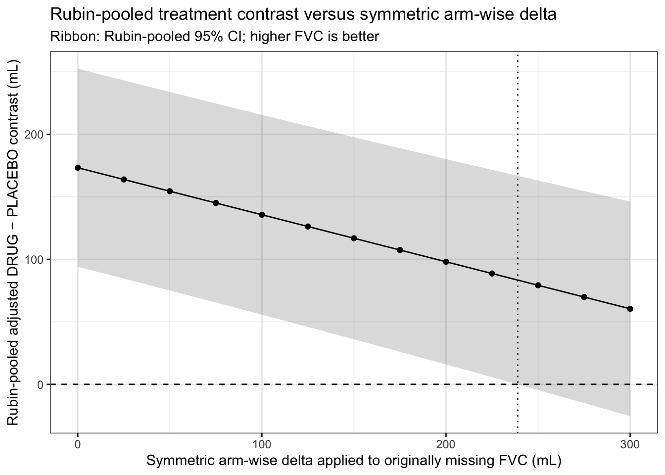

Figure 4: Rubin-pooled adjusted DRUG minus PLACEBO contrast versus symmetric arm-wise delta, with 95% confidence interval.

Step 8 — Two-dimensional tipping surface

A single shared \(\delta\) is only one path through MNAR space: it worsens missing DRUG values and improves missing PLACEBO values by the same amount. The shared-delta analysis should therefore be understood as a deliberately chosen sensitivity path, not as a uniquely defined representation of MNAR. Other clinically plausible assumptions may shift the two treatment arms by different amounts. The two-dimensional analysis makes this dependence visible.

A coarse grid over \((\delta_{\mathrm{DRUG}},\delta_{\mathrm{PLACEBO}})\) shows other combinations that lose or retain the specified statistical criterion (cf. two-way tipping-point displays in Gorst-Rasmussen and Tarp-Johansen, 2022). Each cell is still a full Rubin pool of the 50 imputations.

delta_2d <- seq(0, 300, by = 75)

tip_2d <- expand_grid(delta_drug = delta_2d, delta_pbo = delta_2d) %>%
  pmap_dfr(function(delta_drug, delta_pbo) {
    pool_one_delta(
      imp_data,
      delta_drug = delta_drug,
      delta_pbo  = delta_pbo
    )
  })

ggplot(tip_2d, aes(x = delta_drug, y = delta_pbo, fill = p_one)) +
  geom_tile() +
  geom_text(aes(label = sprintf("%.3f", p_one)), size = 3) +
  geom_abline(slope = 1, intercept = 0, linetype = "dotted") +
  scale_fill_gradient(low = "white", high = "grey30") +
  labs(
    title = "Two-dimensional tipping surface",
    subtitle = "Fill and labels: one-sided p-value; dotted line: shared arm-wise delta path",
    x = "Arm-wise delta applied to originally missing DRUG FVC (mL)",
    y = "Arm-wise delta applied to originally missing PLACEBO FVC (mL)",
    fill = "p (one-sided)"
  ) +
  theme_bw() +
  coord_equal()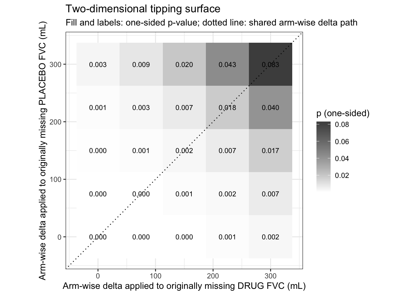

Figure 5: One-sided p-values on a two-dimensional MNAR grid. The dotted diagonal is the shared-delta analysis.

The dotted diagonal is the one-dimensional analysis from Step 6. Cells with \(p \ge 0.025\) are combinations of arm-specific sensitivity shifts for which the specified one-sided statistical criterion is not met. These cells do not establish that the corresponding MNAR assumptions are plausible; they simply identify where the inferential conclusion changes under the chosen sensitivity model.

The two-dimensional surface should also be interpreted as a sensitivity map rather than as an estimate of the probability of different MNAR mechanisms. The axes represent assumed departures from MAR. The analysis does not assign probabilities to those departures.

In practice, the most informative region of the surface is the region containing clinically and scientifically plausible departures from MAR.

Step 9 — Interpretation

tip_results %>%
  transmute(
    delta,
    estimate = round(estimate, 1),
    SE = round(SE, 1),
    df = round(df, 1),
    t = round(t, 2),
    p_one = signif(p_one, 3),
    significant = p_one < alpha_one
  )

# A tibble: 13 × 7
   delta estimate    SE    df     t     p_one significant
   <dbl>    <dbl> <dbl> <dbl> <dbl>     <dbl> <lgl>      
 1     0    173.   40.1  139.  4.32 0.0000146 TRUE       
 2    25    164.   40.1  139.  4.09 0.0000367 TRUE       
 3    50    154.   40.2  140.  3.85 0.0000906 TRUE       
 4    75    145.   40.3  140.  3.6  0.000218  TRUE       
 5   100    136.   40.4  140.  3.36 0.000509  TRUE       
 6   125    126.   40.6  141.  3.11 0.00114   TRUE       
 7   150    117.   40.9  142.  2.86 0.00246   TRUE       
 8   175    108.   41.2  142.  2.61 0.00504   TRUE       
 9   200     98    41.6  144.  2.36 0.00983   TRUE       
10   225     88.6  42    145.  2.11 0.0182    TRUE       
11   250     79.2  42.4  146.  1.87 0.0318    FALSE      
12   275     69.8  42.9  147   1.63 0.0528    FALSE      
13   300     60.4  43.4  148.  1.39 0.0831    FALSE

tp_txt <- if (is.finite(delta_tp_exact)) {
  paste0(round(delta_tp_exact, 1), " mL")
} else {
  "not reached on the explored grid"
}

cat(
  "MAR (delta = 0): estimate = ",
  round(mar_result$estimate, 1),
  " mL, one-sided p = ",
  signif(mar_result$p_one, 3),
  ".\n",
  "Numerical crossing of one-sided criterion (symmetric arm-wise path): approximately ",
  tp_txt,
  ".\n",
  "Overall endpoint missingness: ",
  round(100 * p_miss_overall, 1),
  "%.\n",
  sep = ""
)

MAR (delta = 0): estimate = 173.3 mL, one-sided p = 1.46e-05.
Numerical crossing of one-sided criterion (symmetric arm-wise path): approximately 238.9 mL.
Overall endpoint missingness: 19.5%.

Reading the results:

MAR analysis (\(\delta=0\)). Under the specified MAR imputation model and the pre-specified ANCOVA, the Rubin-pooled DRUG-versus-PLACEBO contrast is reported above with its one-sided \(p\)-value. Under this simulated dataset, the one-sided statistical criterion is therefore assessed under MAR.
Meaning of delta. Each delta value is an arm-wise shift applied only to originally missing endpoint observations. Along the one-dimensional sensitivity path used here, missing DRUG values are decreased by \(\delta\) and missing PLACEBO values are increased by \(\delta\).
Tipping point. In this example, \(\delta_{\mathrm{TP}}\) is the approximate value along the symmetric arm-wise sensitivity path at which the one-sided test crosses the pre-specified significance threshold \(\alpha=0.025\). Values below this boundary retain statistical significance under the specified sensitivity model, while values above it do not.

This is not a boundary between efficacy and no efficacy. For example, at \(\delta=250\) mL the estimated treatment effect remains positive, but its confidence interval includes zero and the one-sided \(p\)-value exceeds 0.025.

The result therefore answers a narrower question: how large would the specified departure from MAR have to be before the pre-specified statistical conclusion changes?
Interpretation of the numerical crossing. The reported value (approximately 238.9 mL in this seed) is an arm-wise outcome shift, not a change of that magnitude in the treatment effect. Under this sensitivity path, it means that each originally missing DRUG endpoint is shifted downward by that amount relative to its MAR-imputed value, while each originally missing PLACEBO endpoint is shifted upward by the same amount.

The resulting ANCOVA treatment contrast at the boundary is much smaller than the arm-wise delta. This is expected because the delta is applied only to originally missing observations and because the final treatment contrast is estimated through the ANCOVA model.
Gender. SEX is a factor in the mice predictor matrix and in lm(FVC_tp ~ TRT + FVC_bl + SEX). The pooled TRTDRUG coefficient is therefore a baseline- and gender-adjusted contrast, not a raw mean difference that ignores the larger male FVC.
Statistical versus clinical conclusion. The tipping point marks loss of the specified statistical criterion, not disappearance of treatment benefit. A separate clinically meaningful threshold could therefore be used to define a clinical rather than purely statistical tipping point.
Plausibility. The practical interpretation depends on whether a departure of that magnitude from the MAR-imputed outcomes is scientifically and clinically plausible. A large numerical tipping point is not automatically evidence of robustness unless the magnitude is meaningful relative to subject-level outcome variability and clinical expectations.
Scope of the conclusion. The result applies only to the specified imputation model, delta-adjustment rule, analysis model, inferential criterion, and sensitivity path. Other plausible MNAR assumptions—particularly asymmetric shifts between treatment arms—can produce different tipping boundaries. The exercise does not prove that missing data are MAR. Observed FVC values are never shifted.

How to specify the sensitivity analysis

A reproducible analysis description should state:

Primary estimand and treatment contrast.
Primary analysis model.
Missingness/imputation model.
Which observations are eligible for delta adjustment.
Direction of the delta adjustment in each arm.
Whether delta is arm-wise or contrast-wise.
The range and increments of the sensitivity parameter.
The rationale for the explored range.
The inferential criterion defining the tipping boundary.
How MI variance and degrees of freedom are combined.
Whether the tipping point is reported as a grid interval or numerical crossing.
How clinical plausibility of the sensitivity range will be assessed.

Take-home message

A multiple-imputation tipping-point analysis is not simply a matter of subtracting a number from the treatment effect. The sensitivity parameter must first be defined as a specific departure applied to originally missing outcomes. Each sensitivity value is then applied separately to every imputed dataset, the primary analysis model is refitted, and the resulting treatment contrasts are Rubin-pooled.

The resulting tipping point is conditional on the chosen sensitivity path and inferential criterion. In particular, an arm-wise delta is not generally equal to the change in an adjusted treatment effect.

The most useful interpretation is therefore not:

“The treatment effect is robust up to 239 mL.”

but:

“Under the specified sensitivity model, the one-sided statistical conclusion remains significant until an arm-wise departure of approximately 239 mL from the MAR-imputed outcomes is imposed on the originally missing observations.”

Whether that represents reassuring robustness depends on whether such a departure from MAR is considered plausible.

References

Missing-data mechanisms and multiple imputation

Rubin, D. B. (1976). Inference and missing data. Biometrika, 63(3), 581–592. https://doi.org/10.1093/biomet/63.3.581
Rubin, D. B. (1987). Multiple Imputation for Nonresponse in Surveys. Wiley.
Barnard, J., and Rubin, D. B. (1999). Small-sample degrees of freedom with multiple imputation. Biometrika, 86(4), 948–955. https://doi.org/10.1093/biomet/86.4.948
van Buuren, S. (2018). Flexible Imputation of Missing Data. 2nd ed. Chapman & Hall/CRC.
van Buuren, S., and Groothuis-Oudshoorn, K. (2011). mice: Multivariate Imputation by Chained Equations in R. Journal of Statistical Software, 45(3), 1–67. https://doi.org/10.18637/jss.v045.i03

Delta-adjustment and tipping-point sensitivity

Yan, X., Lee, S., and Li, N. (2009). Missing data handling methods in medical device clinical trials. Journal of Biopharmaceutical Statistics, 19(6), 1085–1098. https://doi.org/10.1080/10543400903243009
Ratitch, B., O’Kelly, M., and Tosiello, R. (2013). Missing data in clinical trials: from clinical assumptions to statistical analysis using pattern mixture models. Pharmaceutical Statistics, 12(6), 337–347. https://doi.org/10.1002/pst.1549
Cro, S., Morris, T. P., Kenward, M. G., and Carpenter, J. R. (2020). Sensitivity analysis for clinical trials with missing continuous outcome data using controlled multiple imputation: a practical guide. Statistics in Medicine, 39(21), 2815–2842. https://doi.org/10.1002/sim.8569
Gorst-Rasmussen, A., and Tarp-Johansen, M. J. (2022). Fast tipping point sensitivity analyses in clinical trials with missing continuous outcomes under multiple imputation. Journal of Biopharmaceutical Statistics, 32(6), 942–953. https://doi.org/10.1080/10543406.2022.2058525

Regulatory context

ICH E9(R1) emphasizes that sensitivity analyses should assess the robustness of conclusions to assumptions underlying the chosen estimand and estimator, including assumptions concerning missing data. Tipping-point analyses are one useful approach for illustrating how conclusions change under specified departures from the primary missing-data assumptions. They should be interpreted as sensitivity analyses rather than as evidence that a particular MNAR mechanism is true.

National Research Council (2010). The Prevention and Treatment of Missing Data in Clinical Trials. National Academies Press. https://doi.org/10.17226/12955
ICH (2019). ICH E9(R1) Addendum on Estimands and Sensitivity Analysis in Clinical Trials. International Council for Harmonisation.

Footnotes

Missing at random (Rubin, 1976): missingness depends on observed data, not on the unobserved values themselves.↩︎
Missing not at random↩︎
Analysis Of Variance↩︎
Intent To Treat↩︎
Forced Vital Capacity↩︎

Introduction

Example setting

Delta adjustment

What \(\delta\) can mean

Why an arm-wise \(\delta\) is not a \(\delta\) change in \(\Delta\)

What should be stated clearly

Why every imputed dataset must be adjusted separately

The statistical procedure

Step 1 — Analyze each imputed dataset

Step 2 — Rubin pooling

One-sided p-value

What is the tipping point?

Statistical versus clinical tipping points

What the tipping point does NOT tell you

R implementation

Extract all imputed datasets

Delta adjustment

Analyze each imputed dataset

Pool the 50 analyses for one delta

Obtain the one-sided p-value

Run the complete tipping-point grid

Find the tipping point numerically

One more subtle issue: ANOVA vs treatment contrast

The complete conceptual picture

Worked example: simulated FVC trial

Setup

Step 1 — Simulate complete FVC data

Step 2 — Impose MAR missingness on endpoint FVC

Step 3 — Describe the incomplete data

Step 4 — MAR multiple imputation with mice

Step 5 — Analysis and pooling helpers

Step 6 — One-dimensional tipping-point grid

Step 7 — Tipping-point graphics

Step 8 — Two-dimensional tipping surface

Step 9 — Interpretation

How to specify the sensitivity analysis

Take-home message

References

Missing-data mechanisms and multiple imputation

Delta-adjustment and tipping-point sensitivity

Regulatory context

Footnotes

Step 4 — MAR multiple imputation with `mice`