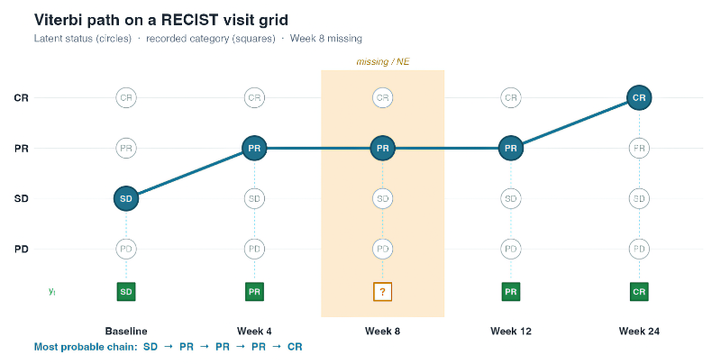
The most probable RECIST-like path when visits go missing
R
Clinical Trials
Data analysis
Missing Data
Data Imputation
Survival
RECIST
Markov-Chain
Author
Vladimir Larchenko
Published
September 21, 2026
Viterbi path on a RECIST visit grid
Introduction
Oncology trials record tumour response on a visit calendar: Baseline \(\rightarrow\) Week 4 \(\rightarrow\) Week 8 \(\rightarrow\) Week 12 \(\rightarrow\) Week 24. At each post-baseline assessment the category is one of CR, PR, SD, or PD.1 Scans are missed, windows are missed, and a visit is coded NE.2 The table then looks like
Last observation carried forward (LOCF) fills the hole with PR. Copying the neighbour on either side does the same. Neither method asks whether the completed chain is a plausible disease course.
A hidden Markov model (HMM) treats the recorded category as a noisy or incomplete view of a latent status \(s_t\) (Baum and Petrie, 1966; Rabiner, 1989). The Viterbi algorithm (Viterbi, 1967; Forney, 1973) returns the single most probable state sequence given the recordings — the MAP3 path, not a visit-wise majority vote.
Restore the chain \(s_1 \rightarrow \cdots \rightarrow s_T\) that maximises \(P(s_{1:T} \mid y_{1:T})\), subject to clinical transition structure (PD absorbing, improvement SD \(\to\) PR \(\to\) CR allowed) and to whatever was actually seen.
This article implements that decoder from scratch in R, on a five-visit RECIST-like grid, including missing visits, unequal spacing, and a short misclassification extension.
A RECIST caveat, stated first. Under RECIST 1.1, Baseline is the reference measurement, not a response category (Therasse et al., 2000; Eisenhauer et al., 2009). CR/PR/SD/PD are defined post-baseline against baseline and nadir; confirmation rules and the 20% + 5 mm PD criterion are operational, not Markov. The five-point chain below is a latent status process on the visit calendar — a reconstruction and QC tool. It is not a best overall response (BOR) engine and must not replace the protocol estimand (ICH E9(R1), 2019).
The following objects are masked from 'package:tidyr':

    expand, pack, unpack
Attaching package: 'expm'
The following object is masked from 'package:Matrix':

    expm
Motivation
Suppose Week 8 is missing and the recorded sequence is SD, PR, NA, PR, CR. In practice the chain gets completed three ways:
Method
Completed chain
LOCF
SD \(\to\) PR \(\to\)PR\(\to\) PR \(\to\) CR
Copy next
SD \(\to\) PR \(\to\)PR\(\to\) PR \(\to\) CR
Independent draw
whatever the marginal at Week 8 suggests
LOCF and copy-next agree here only because the recordings flanking the hole are both PR; they part ways as soon as the next observation differs from the last.
LOCF is a poor primary analysis for longitudinal means (Siddiqui, Hung, and O’Neill, 2009; National Research Council, 2010; Little et al., 2012). For a categorical disease course it fails a second way: it ignores transition constraints. A sequence PD, NA, CR becomes PD, PD, CR under LOCF, which contradicts absorbing progression. Independent imputation of each visit can invent the same impossibility.
Rabiner (1989) separates three HMM jobs:
likelihood of the recordings given the model;
decoding — the most probable state sequence (Viterbi);
learning the parameters (Baum–Welch / EM; Baum et al., 1970).
This post is job 2. Job 3 is out of scope: the transition matrix here is protocol-structured, not estimated from the same small trial we then “complete”.
The decoding estimand is a path. The forward–backward algorithm gives the visit-wise posteriors \[P(S_t = s \mid y_{1:T}),\] yet the visit-wise modes can disagree with the Viterbi path (Rabiner, 1989; Cappé, Moulines, and Rydén, 2005). For “what was the most plausible course of disease?” the path is the right object.
An HMM on the visit grid
Four latent statuses, in clinical order of worsening. The plate below is the same five-visit calendar: a Markov chain of hidden statuses \(s_t\) and a recording \(y_t\) that may be missing.
%%{init: {"theme": "base", "themeVariables": {"darkMode": false, "background": "#ffffff", "primaryColor": "#d6eaf8", "primaryTextColor": "#1a252f", "primaryBorderColor": "#1f6f8b", "lineColor": "#2c3e50", "mainBkg": "#d6eaf8", "clusterBkg": "#f7f9fb", "clusterBorder": "#5d6d7e", "titleColor": "#1a252f"}, "flowchart": {"padding": 12, "nodeSpacing": 18, "rankSpacing": 40, "curve": "linear"}}}%%
flowchart LR
  subgraph hidden [Latent status]
    S0["s1"]
    S1["s2"]
    S2["s3"]
    S3["s4"]
    S4["s5"]
    S0 --> S1 --> S2 --> S3 --> S4
  end
  subgraph rec [Recorded RECIST]
    Y0["y1"]
    Y1["y2"]
    Y2["y3 missing"]
    Y3["y4"]
    Y4["y5"]
  end
  S0 --> Y0
  S1 --> Y1
  S2 --> Y2
  S3 --> Y3
  S4 --> Y4
  classDef hid fill:#d6eaf8,stroke:#1f6f8b,color:#1a252f,stroke-width:1.5px
  classDef seen fill:#d5f5e3,stroke:#1e8449,color:#1a252f,stroke-width:1.5px
  classDef miss fill:#fdebd0,stroke:#b9770e,color:#1a252f,stroke-width:1.8px
  class S0,S1,S2,S3,S4 hid
  class Y0,Y1,Y3,Y4 seen
  class Y2 miss
states <-c("CR", "PR", "SD", "PD")
Visits \(t = 1,\ldots,5\) sit at Baseline, Week 4, Week 8, Week 12, and Week 24. The latent process is a Markov chain
Rows are origin \(s'\), columns destination \(s\), so the entry is \(P(s \mid s')\). PD is absorbing: once progressed, stay PD. Improvement SD \(\to\) PR \(\to\) CR is allowed; CR \(\to\) PR is the confirmation / relapse leak, not a typical recovery from PD.
The last hop on the calendar is 12 weeks, not 4. The matrix above is a 4-week step. Week 12 \(\to\) Week 24 is handled later with a generator \(Q\) and \(P(\Delta t) = \exp(Q\,\Delta t)\) (Kalbfleisch and Lawless, 1985). Until then, treat \(P\) as the one-step kernel on the discrete visit index, which is already enough to see Viterbi work.
Emissions: hard constraints and missing visits
The teaching model makes the recording exact:
if \(y_t = k\) is observed in \(\{\mathrm{CR},\mathrm{PR},\mathrm{SD},\mathrm{PD}\}\), then \(e_t(s) = 1\{s = k\}\) (the recording is the state);
if the visit is missing or NE, \(e_t(s) = 1\) for every \(s\) (the Markov prior fills the gap).
Schwartz et al. (2016) clarify NE / unevaluable under RECIST 1.1; here NE is simply “no emission constraint”. The Noisy emissions section below replaces the indicator with a confusion matrix \(C_{s,k} = P(y=k \mid s)\) (Jackson et al., 2003).
There are \(4^5 = 1024\) chains on five visits — enumerable, but the point of the algorithm is the recurrence that stays \(O(T |S|^2)\) when \(T\) or \(|S|\) grows (Durbin, Eddy, Krogh, and Mitchison, 1998).
Let \(dp_t(s)\) be the probability of the most probable chain that ends in \(s\) at visit \(t\) and that accounts for \(y_{1:t}\). Then (Viterbi, 1967; Forney, 1973; Rabiner, 1989)
If every candidate is impossible, \(\log dp_T = -\infty\): the recorded sequence is incompatible with \(P\) (typically PD then CR under an absorbing kernel).
A three-visit calculation by hand
Take \(y = (\mathrm{SD},\; \mathrm{NA},\; \mathrm{PR})\) and the matrices above. Visit 1 is pinned to SD:
The surviving path is forced at the ends (SD, ?, PR). The missing middle is the \(s'\) that attains the max into PR. Staying in SD at the hole wins: \(P(\mathrm{SD} \mid \mathrm{SD}) = 0.70\) so \(\log dp_2(\mathrm{SD})\) is far above \(\log dp_2(\mathrm{PR})\), and that occupancy beats \(P(\mathrm{PR} \mid \mathrm{PR}) = 0.60\) versus \(P(\mathrm{PR} \mid \mathrm{SD}) = 0.18\). The Viterbi chain is SD \(\to\)SD\(\to\) PR — the same fill LOCF would have written, for a different reason (the kernel, not a copy rule). A more sticky \(P(\mathrm{PR} \mid \mathrm{PR})\) would flip the backpointer.
The recurrence is written once, against a list of one-step kernels — one per hop, P_list[[t - 1]] carrying hop \(t - 1 \to t\). The homogeneous decoder is the special case of feeding the same \(P\) to every hop. We will cash in that generality in the Unequal spacing section.
feasible = FALSE is the honest answer when the recordings contradict the kernel (hard PD then CR). which.max() on a row of \(-\infty\) would otherwise invent a traceback.
Five visits, one hole
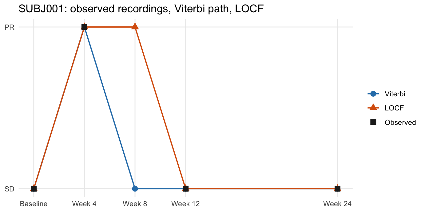
ADaM-style long data: USUBJID, VISIT, TIME, AVALC in {CR, PR, SD, PD, NA}. Subject SUBJ001 is the teaching sequence with a hole at Week 8. A few neighbours are simulated from the same \((\pi, P)\) with MAR-like missingness after Baseline.
On this particular hole LOCF and Viterbi agree. They need not. Replace the Week-12 recording with SD and Viterbi prefers an SD middle; LOCF still copies PR.
Week 12 \(\to\) Week 24 is three times a 4-week step. Treating that hop like any other understates the chance the disease moved during the long gap. What exactly “treating it like any other” means comes in two flavors, and we will compare both against the honest one.
From a step kernel to a holding kernel
A continuous-time Markov chain (CTMC) describes the process with a generator \(Q\) instead of a step matrix: off-diagonal \(q_{ij} \ge 0\) is the instantaneous rate of jumping from state \(i\) to state \(j\) “per week”, the diagonal is \(-q_i\), the rate of leaving state \(i\) altogether, so rows sum to 0, and an absorbing PD is the all-zero row (\(Q_{\mathrm{PD},\cdot} = 0\)). The transition kernel over an interval \(\Delta t\) is then the matrix exponential
\[
P(\Delta t) = \exp(Q\,\Delta t)
\]
(Kalbfleisch and Lawless, 1985; Jackson, 2011). The longer the visit gap, the further \(P(\Delta t)\) moves from the identity: more time to leave every state. Compute the exponential with a proper algorithm, not a truncated series (Moler and Van Loan, 2003); expm::expm() implements Pade with scaling and squaring.
A natural first move is to recover \(Q\) from the protocol \(P\) as a matrix logarithm, \(Q = \log(P)/4\), so that \(P(4) = P\) exactly, and then let \(P(12) = \exp(3 \cdot 4\,Q)\). This does not work here:
The off-diagonal entry \(q_{\mathrm{SD},\mathrm{CR}} < 0\) disqualifies \(\log(P)/4\) as a generator: this \(P\) is a step kernel that is not embeddable in a CTMC — a 4-week step SD \(\to\) CR is allowed, but not as a rate of crossing SD to CR directly. (Embeddability is a real constraint, not a curiosity: a matrix can be a fine one-step kernel and still have no valid generator.) So \(Q\) below is its own expert structure, chosen so that \(P(4)\) resembles the protocol \(P\) — within \(\pm 0.05\) per entry — while rows sum to 0 and PD stays absorbing:
Over 12 weeks the chain has more time to leave CR/PR/SD for PD; the PD row stays \((0,0,0,1)\). The cash-in from the Implementation section: viterbi_tv was built for a list of kernels, so the time-inhomogeneous decoder is just the call — \(P_t = P(\Delta t_t)\) at each hop instead of a single \(P\):
Two shortcuts to the same 12-week hop are tempting, and both misplace probability relative to \(P(\Delta t)\):
use \(P\) once anyway: pretends the gap is 4 weeks; too little time to move, so movement is forced earlier in the calendar than the data warrant;
apply \(P\) three times (\(P^3\)): gets the total time roughly right but enforces a hidden rhythm — three exactly-4-week transitions, with a hold at Weeks 16 and 20 that no scan ever visited; its 12-week holding probabilities differ from \(P(12)\)’s entry by entry (e.g. CR \(\to\) CR 0.41 vs 0.37; SD \(\to\) SD 0.42 vs 0.47).
For SUBJ001 all three decode the same hole as PR, so we add one chain where the choices disagree — SD, PR, --, --, PD — two holes, one long, and a terminal PD:
P3 <- P %*% P %*% Pdimnames(P3) <-dimnames(P)spacing_table <-function(y) { runs <-list(`P once each hop`=list(P, P, P, P),`P^3 on the long hop`=list(P, P, P, P3),`exp(Q dt)`=list(P4, P4, P4, P12) ) out <-map(runs, \(rl) viterbi_tv(y, rl, pi0, emission_hard))tibble(kernel =names(runs),path =map_chr(out, \(o) paste0(o$path, collapse =" ")),feasible =map_lgl(out, \(o) o$feasible),log_prob =map_dbl(out, \(o) o$log_prob) )}spacing_table(y001)
# A tibble: 3 × 4
  kernel              path           feasible log_prob
  <chr>               <chr>          <lgl>       <dbl>
1 P once each hop     SD PR PR PR CR TRUE        -4.99
2 P^3 on the long hop SD PR PR PR CR TRUE        -4.66
3 exp(Q dt)           SD PR PR PR CR TRUE        -5.06
# A tibble: 3 × 4
  kernel              path           feasible log_prob
  <chr>               <chr>          <lgl>       <dbl>
1 P once each hop     SD PR PD PD PD TRUE        -5.07
2 P^3 on the long hop SD PR PR PR PD TRUE        -4.95
3 exp(Q dt)           SD PR PR PR PD TRUE        -4.75
Two things fall out of the second chain. \(P\)-once says progression already by Week 8 (SD PR PD PD PD); \(P^3\) and \(P(\Delta t)\) say stable, then PD at 24 — the naive kernel, which cannot move much per hop, pushes the move earlier and calls it done. And on the first chain the log-likelihoods separate: the same path is \(-4.99\) under \(P\)-once but \(-4.66\) under \(P^3\), so the shortcuts disagree about plausibility even when they agree about the path — which matters as soon as you score or compare chains.
The starkest disagreement is on CR, --, --, --, PD: \(P\)-once decodes it as CR PD PD PD PD (log-prob \(-6.91\)) — progression forced all the way by Week 4 — while \(P(\Delta t)\) decodes it as CR CR CR CR PD (\(-5.99\)): hold CR across the short hops and let the long gap do the moving. The single-4-week kernel, marched across a 12-week gap hop by hop, cannot say “the state is unknown because the interval was long”; it has to over-explain the movement somewhere. On irregular real calendars \(P(\Delta t)\) is the honest discrete skeleton of a continuous-time chain; msm fits that model from panel data (Jackson, 2011).
Noisy emissions
Independent review and local investigators disagree. A recorded PR can be a true CR or SD. Jackson et al. (2003) put that misclassification in the emission; Jackson and Sharples (2002) is the clinical HMM cousin (staged decline, noisy marker).
Let \(C_{s,k} = P(y = k \mid s)\), rows = true status, columns = recorded category:
SD, PD, CR, CR, CR cannot occur if PD is absorbing and emissions are indicators: \(P(\mathrm{CR} \mid \mathrm{PD}) = 0\) and \(e(\mathrm{CR})\) kills every other state.
The noisy decoder does not walk through absorbing PD into CR. It treats the isolated PD as a likely misrecord of SD (or PR) and keeps a chain that can legally reach the later CRs. The opposite reading — trust PD and treat the CRs as false — is possible only because \(C_{\mathrm{PD},\mathrm{CR}} > 0\); here that path loses.
A small \(\varepsilon\) floor on a hard emission, \(e_t(s) = 1\{s=y_t\}(1-\varepsilon) + \varepsilon/(|S|-1)\), is the same idea with a less interpretable \(C\).
Software in R
The decoder above is the teaching object. Production HMM fitting lives elsewhere:
continuous-time Markov and HMM on irregular visits
Zucchini, MacDonald, and Langrock (2016)
textbook discrete-time HMM in R
None of these is a RECIST engine. They estimate and decode; the clinical kernel is still yours.
When not to use Viterbi here
Primary BOR / ORR / PFS. RECIST 1.1 defines confirmation of CR/PR, nadir, target versus non-target, and PD as 20% + 5 mm (Eisenhauer et al., 2009). Viterbi on a four-state calendar does none of that.
Immunotherapy. iRECIST distinguishes iUPD from iCPD; PD is not absorbing (Seymour et al., 2017). The teaching \(P\) above is wrong for IO trials.
Feeding the path into the primary estimator as if observed. Filled-in statuses are not data (National Research Council, 2010; Little et al., 2012). ICH E9(R1) treats progression and dropout as intercurrent events, not as licence to overwrite \(y_t\).
MNAR after silent PD. A missed Week 8 because the subject progressed and left is not a flat emission (Rubin, 1976). The missingness mechanism then carries information that \(e_t \equiv 1\) discards.
Estimating \(P\) from the same small trial you then complete. Baum–Welch on \(n=80\) with \(T=5\) overfits; the completed chains echo the MLE’s prejudices. Keep \(\pi\) and \(P\) external (historical, SAP-specified) if the decoder is a QC check.
Visit-wise reporting of “the” state. Report the path, or report forward–backward posteriors, but do not mix them without saying which estimand you mean (Rabiner, 1989).
Closing
Method
What it maximises / assumes
Typical failure
LOCF / last non-missing
persistence of the last seen label
PD then CR; ignores \(P\)
Independent imputation
visit-wise margins
incoherent chains
Forward–backward modes
\(\arg\max_s P(S_t=s \mid y)\) at each \(t\)
modes need not form a legal path
Multiple imputation
posterior of a scientific estimand
right for means / ORR; not a single chain
Viterbi
\(\arg\max_{s_{1:T}} P(s_{1:T} \mid y)\)
wrong \(P\) or wrong \(e_t\); not a BOR
Use Viterbi when the scientific sentence is “the most probable course of statuses, given this kernel and these recordings.” Use RECIST machinery for the endpoint; use MMRM / MI / ICH E9(R1) for the treatment-effect estimand; use a confusion-matrix emission when the recording itself is on trial.
References
Algorithm and HMM theory
Viterbi, A. J. (1967). Error bounds for convolutional codes and an asymptotically optimum decoding algorithm. IEEE Transactions on Information Theory, 13(2), 260–269. https://doi.org/10.1109/TIT.1967.1054010
Baum, L. E., and Petrie, T. (1966). Statistical inference for probabilistic functions of finite state Markov chains. Annals of Mathematical Statistics, 37(6), 1554–1563. https://doi.org/10.1214/aoms/1177699147
Baum, L. E., Petrie, T., Soules, G., and Weiss, N. (1970). A maximization technique occurring in the statistical analysis of probabilistic functions of Markov chains. Annals of Mathematical Statistics, 41(1), 164–171. https://doi.org/10.1214/aoms/1177697196
Rabiner, L. R. (1989). A tutorial on hidden Markov models and selected applications in speech recognition. Proceedings of the IEEE, 77(2), 257–286. https://doi.org/10.1109/5.18626
Durbin, R., Eddy, S. R., Krogh, A., and Mitchison, G. (1998). Biological Sequence Analysis: Probabilistic Models of Proteins and Nucleic Acids. Cambridge University Press.
Cappé, O., Moulines, E., and Rydén, T. (2005). Inference in Hidden Markov Models. Springer.
Zucchini, W., MacDonald, I. L., and Langrock, R. (2016). Hidden Markov Models for Time Series: An Introduction Using R. 2nd ed. Chapman and Hall/CRC.
Continuous time and unequal visit spacing
Kalbfleisch, J. D., and Lawless, J. F. (1985). The analysis of panel data under a Markov assumption. Journal of the American Statistical Association, 80(392), 863–871. https://doi.org/10.1080/01621459.1985.10478195
Moler, C., and Van Loan, C. (2003). Nineteen dubious ways to compute the exponential of a matrix, twenty-five years later. SIAM Review, 45(1), 3–49. https://doi.org/10.1137/S00361445024180
Clinical multi-state models and misclassification
Jackson, C. H., and Sharples, L. D. (2002). Hidden Markov models for the onset and progression of bronchiolitis obliterans syndrome in lung transplant recipients. Statistics in Medicine, 21(1), 113–128. https://doi.org/10.1002/sim.886
Jackson, C. H., Sharples, L. D., Thompson, S. G., Duffy, S. W., and Couto, E. (2003). Multistate Markov models for disease progression with classification error. Journal of the Royal Statistical Society: Series D (The Statistician), 52(2), 193–209. https://doi.org/10.1111/1467-9884.00351
Jackson, C. H. (2011). Multi-state models for panel data: the msm package for R. Journal of Statistical Software, 38(8), 1–29. https://doi.org/10.18637/jss.v038.i08
Bartolucci, F., Farcomeni, A., and Pennoni, F. (2013). Latent Markov Models for Longitudinal Data. Chapman and Hall/CRC.
Oncology response criteria
Therasse, P., Arbuck, S. G., Eisenhauer, E. A., Wanders, J., Kaplan, R. S., Rubinstein, L., Verweij, J., Van Glabbeke, M., van Oosterom, A. T., Christian, M. C., and Gwyther, S. G. (2000). New guidelines to evaluate the response to treatment in solid tumors. Journal of the National Cancer Institute, 92(3), 205–216. https://doi.org/10.1093/jnci/92.3.205
Eisenhauer, E. A., Therasse, P., Bogaerts, J., Schwartz, L. H., Sargent, D., Ford, R., Dancey, J., Arbuck, S., Gwyther, S., Mooney, M., Rubinstein, L., Shankar, L., Dodd, L., Kaplan, R., Lacombe, D., and Verweij, J. (2009). New response evaluation criteria in solid tumours: revised RECIST guideline (version 1.1). European Journal of Cancer, 45(2), 228–247. https://doi.org/10.1016/j.ejca.2008.10.026
Schwartz, L. H., Litière, S., de Vries, E., Ford, R., Gwyther, S., Mandrekar, S., Shankar, L., Bogaerts, J., Chen, A., Dancey, J., Hayes, W., Hodi, F. S., Hoekstra, O. S., Huang, E. P., Lin, N., Liu, Y., Mu, R., Rubinstein, L., Therasse, P., … Seymour, L. (2016). RECIST 1.1 — update and clarification: from the RECIST committee. European Journal of Cancer, 62, 132–137. https://doi.org/10.1016/j.ejca.2016.03.081
Seymour, L., Bogaerts, J., Perrone, A., Ford, R., Schwartz, L. H., Mandrekar, S., Lin, N. U., Litière, S., Dancey, J., Chen, A., Hodi, F. S., Therasse, P., Hoekstra, O. S., Shankar, L. K., Wolchok, J. D., Ballinger, M., Caron, T. G., and de Vries, E. G. E. (2017). iRECIST: guidelines for response criteria for use in trials testing immunotherapeutics. The Lancet Oncology, 18(3), e143–e152. https://doi.org/10.1016/S1470-2045(17)30074-8
National Research Council (2010). The Prevention and Treatment of Missing Data in Clinical Trials. National Academies Press. https://doi.org/10.17226/12955
Little, R. J., D’Agostino, R., Cohen, M. L., Dickersin, K., Emerson, S. S., Farrar, J. T., Frangakis, C., Hogan, J. W., Molenberghs, G., Murphy, S. A., Neaton, J. D., Rotnitzky, A., Scharfstein, D., Shih, W. J., Siegel, J. P., and Stern, H. (2012). The prevention and treatment of missing data in clinical trials. New England Journal of Medicine, 367(14), 1355–1360. https://doi.org/10.1056/NEJMsr1203730
Siddiqui, O., Hung, H. M. J., and O’Neill, R. (2009). MMRM vs. LOCF: a comprehensive comparison based on simulation study and 25 NDA datasets. Journal of Biopharmaceutical Statistics, 19(2), 227–246. https://doi.org/10.1080/10543400802609723
ICH (2019). ICH E9(R1) Addendum on Estimands and Sensitivity Analysis in Clinical Trials. International Council for Harmonisation.
Software
Visser, I., and Speekenbrink, M. (2010). depmixS4: an R package for hidden Markov models. Journal of Statistical Software, 36(7), 1–21. https://doi.org/10.18637/jss.v036.i07
Helske, S., and Helske, J. (2019). Mixture hidden Markov models for sequence data: the seqHMM package in R. Journal of Statistical Software, 88(3), 1–32. https://doi.org/10.18637/jss.v088.i03
Goulet, V., Dutang, C., Maechler, M., Firth, D., Shapira, M., and Stadelmann, M. (2021). expm: Matrix Exponential, Log, ‘etc’. R package. https://CRAN.R-project.org/package=expm