library(dplyr, warn.conflicts = FALSE)
library(tidyr)
library(ggplot2)Dynamic Programming for PK Dose Sequences
The PK model supplies the transition; Bellman chooses the doses
R
Clinical Trials
Data analysis
Dose finding
Introduction
A one-compartment intravenous (IV) bolus with known elimination rate constant \(k\) and volume of distribution \(V\) is ordinary pharmacokinetics.1 Superposition writes the concentration after a given sequence of doses (Rowland and Tozer, 2011). Steady state tells you the peak, trough, and average that a repeating regimen will settle to.
Neither object is a policy — a rule that selects which dose to give at each decision point. The clinical question is sequential:
Which dose now, given where the concentration sits, so that the whole remaining trajectory is as close as possible to a target concentration, subject to constraints on dose size and frequency?
We want to minimize a cost function that penalizes both deviations from the target concentration and large doses (which may carry toxicity or inconvenience). This is a finite-horizon control problem. The pharmacokinetic model supplies the state transition — how concentration evolves under a given dose. Dynamic programming (DP) chooses the optimal dose sequence that minimizes total cost over the time horizon (Bellman, 1957; Bertsekas, 2017).
A myopic “greedy” rule that only minimizes the immediate one-step cost can fail: it may lock onto the wrong concentration plateau even when it scores each step with the same stage cost the optimal policy accumulates. DP looks ahead to find a globally better trajectory.
This article implements the optimizer from scratch in R: a one-compartment IV bolus, five dose options, a five-step horizon, greedy versus Bellman, and a tight \(C_{\max}\) cap that removes the loading overshoot.
A clinical caveat, stated first. Parameters here are known exactly. There is no residual error, no interindividual variability, no delayed observation, and no Bayesian update. Therapeutic drug monitoring (TDM) and model-informed precision dosing (MIPD) live in that missing layer (Sheiner et al., 1979; Darwich et al., 2017; Keizer et al., 2018). The lattice below is a teaching control problem. It is not a prescribing rule, not a protocol dose-finding engine, and not software as a medical device. ICH M15 concerns model-informed drug development, not bedside automation of this recurrence (ICH, 2026).
The PK map
Continuous-time one-compartment model
After an IV bolus of dose \(D\) into volume of distribution \(V\), the concentration evolves as
\[ C(t)=\frac{D}{V}\,e^{-kt}, \qquad \text{where}\quad k=\frac{\ln 2}{t_{1/2}} \]
is the elimination rate constant. For a half-life \(t_{1/2}=12\,\mathrm{h}\), we have \(k\approx 0.0578\,\mathrm{h}^{-1}\).
Discrete-time dosing epochs
Suppose we make dosing decisions at fixed intervals \(\Delta t=12\,\mathrm{h}\) — once per half-life. Between decisions, the drug is eliminated. The interval elimination factor is
\[ r=e^{-k\Delta t}=e^{-\ln 2}=\tfrac12. \]
This says: concentration halves over one dosing interval in the absence of new doses.
The transition map
Let \(C_t\) denote the concentration at epoch \(t\) (immediately after the dose at that epoch). A dose \(D_t\) chosen at epoch \(t\) arrives at the start of epoch \(t+1\); the concentration then is
\[ C_{t+1} = r\,C_t + \frac{D_t}{V}, \]
where the first term accounts for elimination and the second for the instantaneous bolus. We abbreviate \(C_{t+1}\) as \(C'\) when the time index is clear.
Parameters and action set
With \(V=50\,\mathrm{L}\), a \(100\,\mathrm{mg}\) bolus raises \(C\) by \(2\,\mathrm{mg/L}\). We restrict doses to a discrete set:
\[ D\in\mathcal{D}=\{0,100,200,300,400\}\,\mathrm{mg}, \qquad u=\frac{D}{V}\in\{0,2,4,6,8\}\,\mathrm{mg/L}. \]
Here \(u\) is the concentration increment from a bolus. The planning horizon is \(H=5\) epochs, and we start from \(C_0=0\).
half_life <- 12
dt <- 12
V <- 50
r <- exp(-log(2) * dt / half_life)
target <- 5
lambda <- 0.02
doses <- c(0, 100, 200, 300, 400)
H <- 5
c0 <- 0

pk_next <- function(c, dose) r * c + dose / V

stage_cost <- function(c_next, dose) {
  u <- dose / V
  (c_next - target)^2 + lambda * u^2
}

c(r = r, V = V, target = target, lambda = lambda, H = H)
#>      r      V target lambda      H
#>   0.50  50.00   5.00   0.02   5.00
The PK model does not choose \(D\). It only answers: given this \(C\) and this \(D\), where do we land. The dosing policy comes from optimizing a cost function over multiple steps.
The cost function and objective
We want the concentration trajectory to stay close to a target \(C_{\mathrm{target}}=5\,\mathrm{mg/L}\) over the five epochs. The dose chosen at epoch \(t\) lands in the state \(C_{t+1}\), so the stage cost \(L(C_{t+1},D_t)\) incurred there penalizes:
- Deviation from target: \((C_{t+1} - C_{\mathrm{target}})^2\), squared to penalize large deviations more heavily.
- Dose magnitude: \(\lambda u_t^2\) where \(u_t=D_t/V\), to discourage unnecessarily large boluses (\(\lambda=0.02\) is a small weight).
The stage cost is therefore
\[ L(C',D) = (C' - 5)^2 + 0.02\,\left(\frac{D}{V}\right)^2, \]
where \(C'\) is the post-dose concentration after giving \(D\). The total cost of a dose sequence \((D_0,D_1,\ldots,D_{H-1})\) is
\[ \text{Total cost} = \sum_{t=0}^{H-1} L(C_{t+1}, D_t), \]
where \(C_{t+1}=r C_t + D_t/V\) under the PK transition. Our goal is to find the dose sequence that minimizes this total cost.
The PK-DP feedback loop
The interplay between the PK model and the DP optimization can be visualized as a feedback loop at each epoch:
%%{init: {"theme": "base", "themeVariables": {"darkMode": false, "background": "#ffffff", "primaryColor": "#d6eaf8", "primaryTextColor": "#1a252f", "primaryBorderColor": "#1f6f8b", "lineColor": "#2c3e50", "mainBkg": "#d6eaf8", "clusterBkg": "#f7f9fb", "clusterBorder": "#5d6d7e", "titleColor": "#1a252f"}, "flowchart": {"padding": 12, "nodeSpacing": 22, "rankSpacing": 36, "curve": "linear"}}}%%
flowchart LR
  subgraph pk [PK transition]
    Cnow["$$C_t$$"]
    Cnext["$$C' = r\cdot C + D/V$$"]
    Cnow --> Cnext
  end
  subgraph dp [DP choice]
    Doses["D in the discrete set"]
    Cost["min L plus  $$\:V_{t+1}$$"]
    Doses --> Cost
  end
  Cost --> Cnext
  classDef hid fill:#d6eaf8,stroke:#1f6f8b,color:#1a252f,stroke-width:1.5px
  classDef pkc fill:#d5f5e3,stroke:#1e8449,color:#1a252f,stroke-width:1.5px
  class Cnow,Cnext pkc
  class Doses,Cost hid
How to read this diagram:
At each decision epoch \(t\), the process unfolds as follows:
Current state (left green box): We observe the current concentration \(C_t\) at epoch \(t\).
PK transition (right green box): The pharmacokinetic model gives us a transition function \(C' = r\cdot C_t + D/V\). This is pure science — it describes how concentration evolves under elimination and dosing. The PK model does not tell us which dose to choose; it only predicts the outcome of any given dose.
DP decision (left blue box): Dynamic programming considers all possible doses \(D\in\{0,100,200,300,400\}\) from the discrete action set. For each candidate dose, we know where it would take us (via the PK transition).
Cost evaluation (right blue box): For each candidate dose, DP computes the total future cost:
- Immediate cost \(L(C',D)\): how much does landing at \(C'\) cost us at this step?
- Future cost-to-go \(V_{t+1}(C')\): what is the minimum cost achievable from state \(C'\) onward? (This comes from having already solved later epochs backward, or from the forward table we’re building.)
Optimal choice: DP selects the dose \(D\) that minimizes \(L(C',D) + V_{t+1}(C')\). This is the lookahead — it picks the dose whose total cost (immediate plus future) is smallest.
State update (arrow from DP back to PK): The chosen dose is applied, the PK transition computes the new concentration \(C'\), and this becomes \(C_{t+1}\) for the next epoch. The loop repeats.
The key insight: The PK box is deterministic chemistry and physiology. The DP box is optimization — it uses the PK predictions to compare all possible futures and picks the best one. A greedy policy would ignore the \(V_{t+1}\) term and only minimize \(L\) now.
Why greedy is not enough
The greedy policy
A greedy (myopic) policy chooses at each step the dose that minimizes \(L\) for that step alone, ignoring future consequences. Starting from \(C_0=0\), let’s evaluate the one-step cost for each possible first dose:
first_step <- tibble(dose = doses) %>%
  mutate(
    u = dose / V,
    c_next = pk_next(c0, dose),
    sq_err = (c_next - target)^2,
    dose_pen = lambda * u^2,
    L = sq_err + dose_pen
  )
first_step
#> # A tibble: 5 × 6
#>    dose     u c_next sq_err dose_pen     L
#>   <dbl> <dbl>  <dbl>  <dbl>    <dbl> <dbl>
#> 1     0     0      0     25     0    25
#> 2   100     2      2      9     0.08  9.08
#> 3   200     4      4      1     0.32  1.32
#> 4   300     6      6      1     0.72  1.72
#> 5   400     8      8      9     1.28 10.3
Why greedy fails
The squared error component ties \(D=200\,\mathrm{mg}\) (giving \(C'=4\)) and \(D=300\,\mathrm{mg}\) (giving \(C'=6\)): both land \(1\,\mathrm{mg/L}\) away from the target. The dose penalty \(\lambda u^2\) breaks the tie in favor of the smaller dose: \(L=1.32\) for \(D=200\,\mathrm{mg}\) versus \(L=1.72\) for \(D=300\,\mathrm{mg}\).
A greedy policy therefore opens with \(200\,\mathrm{mg}\).
From \(C=4\), half-life elimination gives \(C=2\) before the next dose. Adding \(100\,\mathrm{mg}\) returns \(C=4\). Repeating \(200\,\mathrm{mg}\) would give \(C=6\), which has higher cost than \(C=4\). So greedy locks onto
\[ D=(200,100,100,100,100)\,\mathrm{mg}, \qquad C=(4,4,4,4,4). \]
The discrete-dose trap
For linear kinetics with constant maintenance dose \(u=D/V\), the steady-state concentration is
\[ C_{\mathrm{ss}} = \frac{u}{1-r}. \]
With \(r=0.5\) and \(u=2\) (from \(D=100\,\mathrm{mg}\)), we get \(C_{\mathrm{ss}}=4\), not the target \(5\). To hit \(C_{\mathrm{ss}}=5\) would require \(u=2.5\), hence \(D=125\,\mathrm{mg}\), which is not in our discrete set \(\{0,100,200,300,400\}\).
Greedy picks the best available steady state on the grid, which is \(C=4\). But dynamic programming can do better by exploiting transient behavior.
The five arrows out of \(C=0\):
%%{init: {"theme": "base", "themeVariables": {"darkMode": false, "background": "#ffffff", "primaryColor": "#d6eaf8", "primaryTextColor": "#1a252f", "primaryBorderColor": "#1f6f8b", "lineColor": "#2c3e50", "mainBkg": "#d6eaf8", "clusterBkg": "#f7f9fb", "clusterBorder": "#5d6d7e", "titleColor": "#1a252f"}, "flowchart": {"padding": 10, "nodeSpacing": 16, "rankSpacing": 48, "curve": "linear"}}}%%
flowchart LR
  S["(t, C = 0)"]
  S -->|"0 mg"| A["C' = 0"]
  S -->|"100 mg"| B["C' = 2"]
  S -->|"200 mg"| G["C' = 4 greedy"]
  S -->|"300 mg"| D["C' = 6 DP"]
  S -->|"400 mg"| E["C' = 8"]
  classDef hid fill:#d6eaf8,stroke:#1f6f8b,color:#1a252f,stroke-width:1.5px
  classDef pkc fill:#d5f5e3,stroke:#1e8449,color:#1a252f,stroke-width:1.5px
  classDef greedy fill:#fdebd0,stroke:#b9770e,color:#1a252f,stroke-width:1.8px
  classDef dp fill:#1f6f8b,stroke:#15485a,color:#ffffff,stroke-width:1.8px
  class S hid
  class A,B,E pkc
  class G greedy
  class D dp
The loading overshoot insight
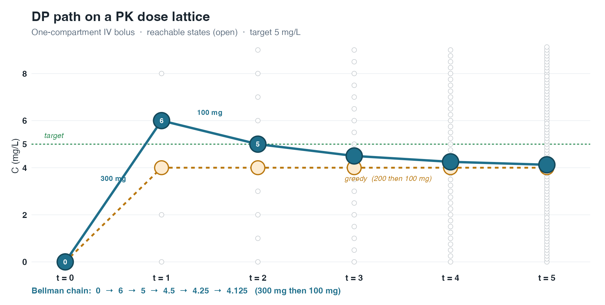
DP asks a different question: what if we pay the higher cost \(L=1.72\) now to reach \(C=6\), accepting the overshoot? After one epoch of elimination, \(C\) drops to \(3\), and adding \(100\,\mathrm{mg}\) gives
\[ C_{t=2} = 0.5\cdot 6 + 2 = 5, \]
hitting the target exactly at \(t=2\). From there, the trajectory decays more slowly through \((5, 4.5, 4.25, 4.125)\) — staying closer to target on average than the greedy path stuck at \(4\).
This is the loading overshoot strategy. Greedy never considers it because \(1.32<1.72\) at the first step; it cannot see that the short-term sacrifice buys a better long-term trajectory.
Bellman’s principle and the DP recurrence
State, action, and transition
A state is \((t,C)\) — the current epoch and concentration. An action is a dose \(D\in\mathcal{D}\). The transition is \(C'=rC+D/V\).
Value function and cost-to-go
Let \(V_t(C)\) denote the minimum achievable cost from epoch \(t\) onward, starting from concentration \(C\) at that epoch. This is called the cost-to-go or value function.
At the terminal epoch \(t=H\), we incur no further cost:
\[ V_H(C) = 0 \quad \text{for all } C. \]
For earlier epochs \(t<H\), Bellman’s principle of optimality states:
\[ V_t(C) = \min_{D\in\mathcal{D}} \Bigl[ \underbrace{L(C',D)}_{\text{immediate cost}} + \underbrace{V_{t+1}(C')}_{\text{future cost-to-go}} \Bigr], \]
where \(C'=rC+D/V\) is the post-dose concentration. This says: the optimal cost-to-go equals the immediate stage cost plus the optimal future cost from the resulting state, minimized over all possible dose choices.
We solve this backward from \(t=H\) down to \(t=0\), building up the optimal policy at each state.
Analogy to other DP problems
This is the same tabular DP pattern as a 0-1 knapsack or longest common subsequence problem, only the meaning of the state changes (here a minimization over all five doses at once, not the knapsack’s binary take-or-skip):
| Question | Knapsack | This PK problem |
|---|---|---|
| What is a state? | (item \(i\), capacity \(w\)) | (epoch \(t\), concentration \(C\)) |
| What is a transition? | take / skip the item | PK map \(C\mapsto C'\) under \(D\) |
| What is terminal? | \(i=0\) or \(w=0\) | \(t=H\), no salvage cost |
Shortest path interpretation
The same recurrence is a shortest path problem on a directed acyclic graph (DAG). Nodes are reachable states \((t,C)\). Each arrow from \((t,C)\) to \((t+1,C')\) represents giving dose \(D\), with edge weight \(L(C',D)\). We seek the cheapest path from the initial state \((0,0)\) to any terminal state \((H,C)\) (Bertsekas, 2017).
Forward versus backward computation
The theoretical formulation above computes \(V_t\) backward from \(t=H\) to \(t=0\). For a DAG, we can equivalently compute cost-to-reach forward from \(t=0\), storing at each node the minimum cumulative cost to reach that state and the predecessor state. After reaching \(t=H\), we backtrack through predecessors to reconstruct the optimal path.
The code below uses forward accumulation — analogous to Viterbi decoding, with \(L\) in place of \(-\log p\). This is sometimes easier to implement and matches the natural left-to-right flow of the dosing timeline.
Implementation in R
Reachable concentrations under this grid stay a sparse set: five nodes after the first dose, then \(13\), \(29\), \(61\), \(125\). A dense mesh in \(C\) is unnecessary. Encode \(C\) by rounding when grouping so that floating keys do not split a state.
reconstruct_path <- function(nodes, H) {
  cur <- nodes %>%
    filter(t == H) %>%
    slice_min(cost, n = 1, with_ties = FALSE)
  acc <- vector("list", H + 1)
  acc[[H + 1]] <- cur
  for (tt in H:1) {
    prev <- nodes %>%
      filter(
        t == tt - 1,
        round(.data$c, 8) == round(cur$prev_c[[1]], 8)
      )
    if (nrow(prev) != 1) {
      stop("predecessor lookup at t=", tt - 1, " matched ",
        nrow(prev), " node(s); states are no longer unique")
    }
    acc[[tt]] <- prev
    cur <- prev
  }
  bind_rows(acc)
}

solve_dose_dp <- function(c_min = -Inf, c_max = Inf) {
  nodes <- tibble(
    t = 0,
    c = c0,
    cost = 0,
    prev_c = NA_real_,
    dose = NA_real_
  )
  for (tt in 0:(H - 1)) {
    layer <- filter(nodes, t == tt)
    expanded <- tidyr::crossing(layer, dose_new = doses) %>%
      mutate(
        c_next = pk_next(c, dose_new),
        cost_next = cost + stage_cost(c_next, dose_new)
      ) %>%
      filter(c_next >= c_min, c_next <= c_max) %>%
      mutate(c_key = round(c_next, 8)) %>%
      group_by(c_key) %>%
      slice_min(cost_next, n = 1, with_ties = FALSE) %>%
      ungroup() %>%
      transmute(
        t = tt + 1,
        prev_c = c,
        c = c_next,
        cost = cost_next,
        dose = dose_new
      )
    nodes <- bind_rows(nodes, expanded)
  }
  list(nodes = nodes, path = reconstruct_path(nodes, H))
}

greedy_policy <- function() {
  c <- c0
  total <- 0
  rows <- vector("list", H)
  for (tt in 1:H) {
    step <- tibble(dose = doses, c_next = pk_next(c, doses)) %>%
      mutate(L = stage_cost(c_next, dose)) %>%
      slice_min(L, n = 1, with_ties = FALSE)
    total <- total + step$L
    rows[[tt]] <- tibble(
      t = tt, c = step$c_next, dose = step$dose, cost = total
    )
    c <- step$c_next
  }
  bind_rows(
    tibble(t = 0, c = c0, dose = NA_real_, cost = 0),
    bind_rows(rows)
  )
}
dp <- solve_dose_dp()
greedy <- greedy_policy()
n_states <- dp$nodes %>%
count(t, name = "n_reachable")
n_states
#> # A tibble: 6 × 2
#> t n_reachable
#> <dbl> <int>
#> 1 0 1
#> 2 1 5
#> 3 2 13
#> 4 3 29
#> 5 4 61
#> 6 5 125
dp$path %>%
transmute(t, dose, C = c, cost)
#> # A tibble: 6 × 4
#> t dose C cost
#> <dbl> <dbl> <dbl> <dbl>
#> 1 0 NA 0 0
#> 2 1 300 6 1.72
#> 3 2 100 5 1.8
#> 4 3 100 4.5 2.13
#> 5 4 100 4.25 2.77
#> 6 5 100 4.12 3.62
greedy %>%
transmute(t, dose, C = c, cost)
#> # A tibble: 6 × 4
#> t dose C cost
#> <dbl> <dbl> <dbl> <dbl>
#> 1 0 NA 0 0
#> 2 1 200 4 1.32
#> 3 2 100 4 2.4
#> 4 3 100 4 3.48
#> 5 4 100 4 4.56
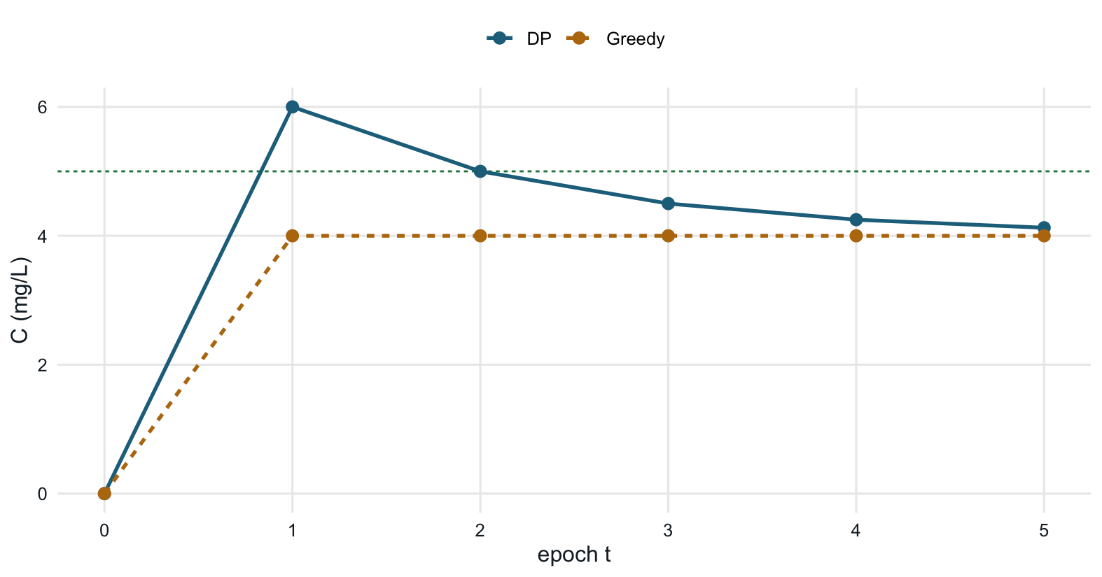
#> 6 5 100 4 5.64DP opens with \(300\,\mathrm{mg}\), visits \(C=6\), then holds \(100\,\mathrm{mg}\). Greedy opens with \(200\,\mathrm{mg}\) and never leaves \(C=4\). After \(t=1\) both policies use the same maintenance dose; the only disagreement is the loading bolus. That is the lookahead.
tibble(
  policy = c("DP (Bellman)", "Greedy (one-step L)"),
  doses = c(
    paste(dp$path$dose[-1], collapse = ", "),
    paste(greedy$dose[-1], collapse = ", ")
  ),
  C_path = c(
    paste(dp$path$c[-1], collapse = ", "),
    paste(greedy$c[-1], collapse = ", ")
  ),
  total_cost = c(last(dp$path$cost), last(greedy$cost))
)
#> # A tibble: 2 × 4
#>   policy              doses                   C_path                 total_cost
#>   <chr>               <chr>                   <chr>                       <dbl>
#> 1 DP (Bellman)        300, 100, 100, 100, 100 6, 5, 4.5, 4.25, 4.125       3.62
#> 2 Greedy (one-step L) 200, 100, 100, 100, 100 4, 4, 4, 4, 4                5.64
Total cost \(3.618\) versus \(5.64\). The extra \(0.40\) paid at the first step (\(1.72\) versus the greedy \(1.32\)) buys a visit to \(C=5\) at \(t=2\) and a slower drift toward the discrete steady state \(4\).
Why does the DP path decay after \(t=2\)? Not because the objective is blind at the endpoint: the final arrival is priced like every other one — the last stage cost is \((4.125-5)^2 + 0.08 = 0.846\), close to a quarter of the total. The decay is the discrete-dose trap at work. Holding \(C=5\) would take \(125\,\mathrm{mg}\) at every epoch; off that dose, from \(C=5\) the only reachable next states are \(\{2.5, 4.5, 6.5, 8.5, 10.5\}\), and \(4.5\) (one \(100\,\mathrm{mg}\) step, cost \(0.33\)) is closest to target. The same comparison recurs at \(4.5\) and \(4.25\) — cheaper to decay a little than to pay for a \(200\,\mathrm{mg}\) swing back up. A terminal penalty \((C_H-5)^2\) prices the endpoint, not the flight path: even when we add it at weight \(1\), brute force over all 3125 sequences still runs the middle of the path through \((6, 5, 4.5)\) before rerouting the last dose to finish at \(5.125\).
col_dp <- "#1F6F8B"
col_greedy <- "#B9770E"
col_target <- "#1E8449"
col_ink <- "#1A252F"

traj <- bind_rows(
  dp$path %>% transmute(t, c, policy = "DP"),
  greedy %>% transmute(t, c, policy = "Greedy")
)

ggplot(traj, aes(t, c, colour = policy, linetype = policy)) +
  geom_hline(
    yintercept = target, colour = col_target, linewidth = 0.5,
    linetype = "22"
  ) +
  geom_line(linewidth = 0.95) +
  geom_point(size = 2.6) +
  scale_colour_manual(values = c(DP = col_dp, Greedy = col_greedy)) +
  scale_linetype_manual(values = c(DP = "solid", Greedy = "22")) +
  scale_x_continuous(breaks = 0:H) +
  labs(x = "epoch t", y = "C (mg/L)", colour = NULL, linetype = NULL) +
  theme_minimal(base_size = 12) +
  theme(
    legend.position = "top",
    panel.grid.minor = element_blank(),
    axis.title = element_text(colour = col_ink),
    axis.text = element_text(colour = col_ink)
  )
Therapeutic window as a hard constraint
Drop any transition with \(C'\) outside \([C_{\min},C_{\max}]\). The solver does not change; the action set becomes state-dependent.
A realistic window for this toy, say \(2\le C'\le 8\), still admits the loading peak of \(6\). The Bellman path is unchanged:
dp_win_wide <- solve_dose_dp(c_min = 2, c_max = 8)
dp_win_wide$path %>%
  transmute(t, dose, C = c, cost)
#> # A tibble: 6 × 4
#>       t  dose     C  cost
#>   <dbl> <dbl> <dbl> <dbl>
#> 1     0    NA  0     0
#> 2     1   300  6     1.72
#> 3     2   100  5     1.8
#> 4     3   100  4.5   2.13
#> 5     4   100  4.25  2.77
#> 6     5   100  4.12  3.62
A tight peak cap \(C_{\max}=5.5\) forbids \(C'=6\) and \(C'=8\) from \(C=0\). The loading overshoot is illegal. DP collapses onto the greedy opening:
dp_win_tight <- solve_dose_dp(c_min = 0, c_max = 5.5)
dp_win_tight$path %>%
  transmute(t, dose, C = c, cost)
#> # A tibble: 6 × 4
#>       t  dose     C  cost
#>   <dbl> <dbl> <dbl> <dbl>
#> 1     0    NA     0  0
#> 2     1   200     4  1.32
#> 3     2   100     4  2.4
#> 4     3   100     4  3.48
#> 5     4   100     4  4.56
#> 6     5   100     4  5.64
That is the clinical reading of the constraint: if the protocol forbids the overshoot that lookahead wanted, the extra future value of \(C=6\) is simply not in the feasible set. The DP path collapses onto the greedy path not because the algorithm changed, but because the loading peak is now illegal.
Hard \(C_{\max}/C_{\min}\) bounds are one way a therapeutic window enters this DP. Soft penalties on excursions are the other, milder, encoding — already present as \((C'-5)^2\) in the stage cost. The trade-off is: hard constraints guarantee safety but may force a suboptimal trajectory; soft penalties allow occasional excursions if the overall cost benefit is large enough.
What this is not
The state here is a scalar \(C\). An oral one-compartment model has \((A_g,A_c)\) and the map needs \(k_a\) as well as \(k_e\). A two-compartment IV model has \((A_c,A_p)\). The Bellman update does not change; the node key becomes a pair, and the lattice grows fast. That is the natural sequel, not this post.
Three other missing pieces, on purpose:
- Unknown \(\theta\). Real MIPD updates \(k\) and \(V\) from measured concentrations (Sheiner et al., 1979; Jelliffe et al., 1993). That is Bayesian forecasting, then a new open-loop plan — or a receding-horizon step of model predictive control (Rawlings, Mayne, and Diehl, 2017).
- Stochastic DP. Interindividual variability and residual error turn \(C'\) into a distribution. Expectation of \(L\) replaces \(L\). The table is then an MDP (Puterman, 1994).
- Continuous \(D\) or free times. A discrete \(D\) on a fixed clock is what makes the DAG small. Optimizing dose and clock is a different mixed-integer problem.
PK model + DP + state estimation is sequential dosing optimization. It is close in spirit to target-concentration intervention (Holford, 1999) and to MIPD. It is not a substitute for either until the error model and the update are there.
When not to use this
- ADaM tables and CSR displays. SDTM/ADaM programming is joins, windows, and estimators — not a Bellman table.
- Protocol dose finding. Phase I/II designs (3+3, CRM, BOIN, MCP-Mod) answer a population question. This lattice answers an individual sequence under a known model.
- Primary TDM in the clinic. Use a residual-error model and a posterior for \(\theta\), then a dose that hits AUC, trough, or \(C_{\mathrm{ss}}\) (Sheiner et al., 1979; Rowland and Tozer, 2011). Vancomycin AUC/MIC workflows are in that family, not in an open-loop five-step DAG with \(\theta\) known.
- Nonlinear PK unless you discretize the state after the nonlinear map. Superposition is gone; the transition is still a function \(f(x,u)\), so DP still applies, but the sparse grid of this toy will not.
- Production MIPD software. Audit, device regulation, and covariate models live elsewhere (Darwich et al., 2017; Keizer et al., 2018; ICH, 2026). The recurrence above is the teaching object you can read.
Closing
| Method | What it optimizes | Typical failure |
|---|---|---|
| Repeat a labeled \(D\) | convenience | wrong \(C_{\mathrm{ss}}\) on a coarse grid |
| Myopic / greedy | one-step \(L\) | skips the loading overshoot |
| Steady-state formula | peak / trough / \(C_{\mathrm{av,ss}}\) | ignores the transient path |
| DP on the PK DAG | \(\sum_t L(C_{t+1},D_t)\) | known \(\theta\); discrete \(D\); no error model |
| Bayesian TDM / MIPD | posterior predictive target | needs data, \(g(\theta)\), and an update |
Use this DP when the scientific sentence is: the PK model supplies the transition, and we want the cheapest feasible dose sequence on a known discrete set. Use superposition and steady-state formulae to understand a fixed regimen. Use TDM / MIPD when \(\theta\) is the patient’s, not the textbook’s.
References
Dynamic programming and control
- Bellman, R. (1957). Dynamic Programming. Princeton University Press.
- Bertsekas, D. P. (2017). Dynamic Programming and Optimal Control. 4th ed. Athena Scientific.
- Puterman, M. L. (1994). Markov Decision Processes: Discrete Stochastic Dynamic Programming. Wiley. https://doi.org/10.1002/9780470316887
- Rawlings, J. B., Mayne, D. Q., and Diehl, M. (2017). Model Predictive Control: Theory, Computation, and Design. 2nd ed. Nob Hill Publishing.
Pharmacokinetics
- Rowland, M., and Tozer, T. N. (2011). Clinical Pharmacokinetics and Pharmacodynamics: Concepts and Applications. 4th ed. Lippincott Williams and Wilkins.
- Gabrielsson, J., and Weiner, D. (2016). Pharmacokinetic and Pharmacodynamic Data Analysis. 5th ed. Swedish Pharmaceutical Press.
- Gibaldi, M., and Perrier, D. (1982). Pharmacokinetics. 2nd ed. Marcel Dekker.
TDM, Bayesian forecasting, and MIPD
- Sheiner, L. B., Beal, S., Rosenberg, B., and Marathe, V. V. (1979). Forecasting individual pharmacokinetics. Clinical Pharmacology and Therapeutics, 26(3), 294–305. https://doi.org/10.1002/cpt1979263294
- Jelliffe, R. W., Schumitzky, A., Van Guilder, M., Liu, M., Hu, L., Maire, P., Gomis, P., Barbaut, X., and Tahani, B. (1993). Individualizing drug dosage regimens: roles of population pharmacokinetic and dynamic models, Bayesian fitting, and adaptive control. Therapeutic Drug Monitoring, 15(5), 380–393. https://doi.org/10.1097/00007691-199310000-00005
- Holford, N. H. G. (1999). Target concentration intervention: beyond Y2K. British Journal of Clinical Pharmacology, 48(1), 9–13. https://doi.org/10.1046/j.1365-2125.1999.00971.x
- Darwich, A. S., Ogungbenro, K., Vinks, A. A., Powell, J. R., Reny, J.-L., Marsousi, N., Daali, Y., Fairman, D., Cook, J., Lesko, L. J., and others (2017). Why has model-informed precision dosing not yet become common clinical reality? Lessons from the past and a roadmap for the future. Clinical Pharmacology and Therapeutics, 101(5), 646–656. https://doi.org/10.1002/cpt.659
- Keizer, R. J., ter Heine, R., Frymoyer, A., Lesko, L. J., Mangat, R., and Goswami, S. (2018). Model-informed precision dosing at the bedside: scientific challenges and opportunities. CPT: Pharmacometrics and Systems Pharmacology, 7(12), 785–787. https://doi.org/10.1002/psp4.12353
- ICH (2026). ICH M15: General Principles for Model-Informed Drug Development. International Council for Harmonisation.
Footnotes
Amount \(A(t)\) in a single well-mixed compartment; \(C=A/V\); first-order elimination \(\mathrm{d}A/\mathrm{d}t=-kA\).↩︎